Scalar (deprecated)
⚠️ Deprecated since 0.23.0: Use Scalars instead.
A double-precision scalar, e.g. for use for time-series plots.
The current timeline value will be used for the time/X-axis, hence scalars should not be static.
When used to produce a plot, this archetype is used to provide the data that
is referenced by archetypes.SeriesLines or archetypes.SeriesPoints. You can do
this by logging both archetypes to the same path, or alternatively configuring
the plot-specific archetypes through the blueprint.
Fields fields
Required required
scalar:Scalar
Can be shown in can-be-shown-in
API reference links api-reference-links
Examples examples
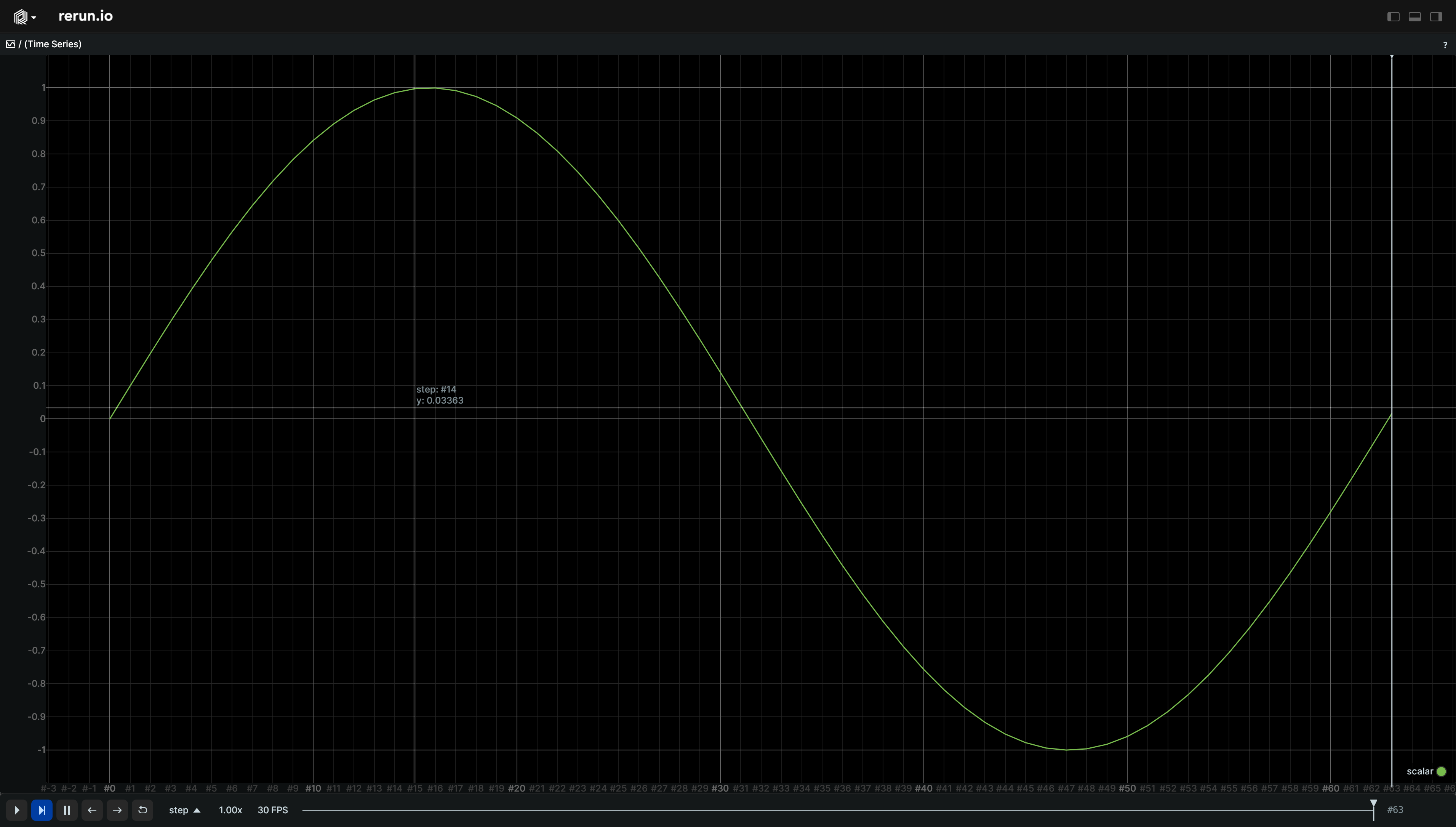
Simple line plot simple-line-plot
"""Log a scalar over time."""

import math

import rerun as rr

rr.init("rerun_example_scalar", spawn=True)

# Log the data on a timeline called "step".
for step in range(64):
    rr.set_time("step", sequence=step)
    rr.log("scalar", rr.Scalars(math.sin(step / 10.0)))
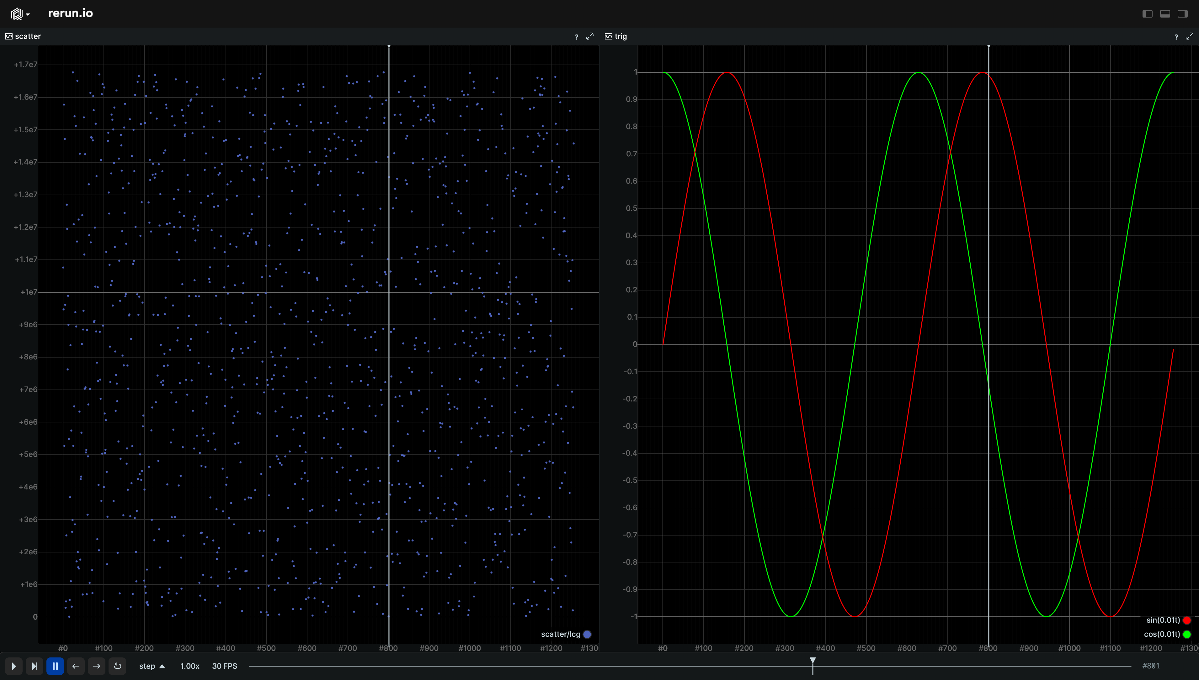
Multiple time series plots multiple-time-series-plots
"""Log a scalar over time."""

from math import cos, sin, tau

import numpy as np
import rerun as rr

rr.init("rerun_example_scalar_multiple_plots", spawn=True)
lcg_state = np.int64(0)

# Set up plot styling:
# They are logged as static as they don't change over time and apply to all timelines.
# Log two lines series under a shared root so that they show in the same plot by default.
rr.log("trig/sin", rr.SeriesLines(colors=[255, 0, 0], names="sin(0.01t)"), static=True)
rr.log("trig/cos", rr.SeriesLines(colors=[0, 255, 0], names="cos(0.01t)"), static=True)
# Log scattered points under a different root so that they show in a different plot by default.
rr.log("scatter/lcg", rr.SeriesPoints(), static=True)

# Log the data on a timeline called "step".
for t in range(int(tau * 2 * 100.0)):
    rr.set_time("step", sequence=t)

    rr.log("trig/sin", rr.Scalars(sin(float(t) / 100.0)))
    rr.log("trig/cos", rr.Scalars(cos(float(t) / 100.0)))

    lcg_state = (1140671485 * lcg_state + 128201163) % 16777216  # simple linear congruency generator
    rr.log("scatter/lcg", rr.Scalars(lcg_state.astype(np.float64)))
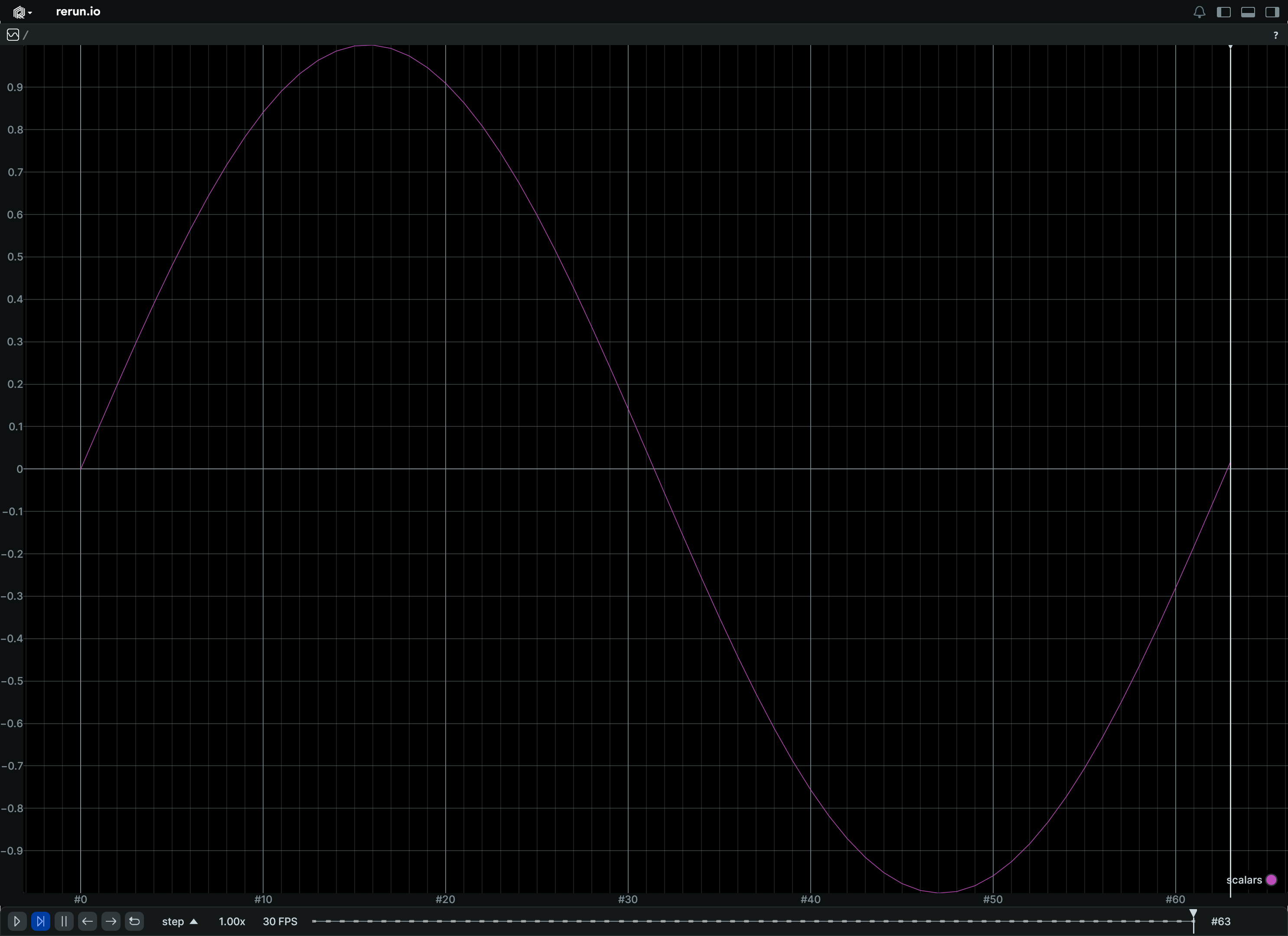
Update a scalar over time update-a-scalar-over-time
"""
Update a scalar over time.

See also the `scalar_column_updates` example, which achieves the same thing in a single operation.
"""

from __future__ import annotations

import math

import rerun as rr

rr.init("rerun_example_scalar_row_updates", spawn=True)

for step in range(64):
    rr.set_time("step", sequence=step)
    rr.log("scalars", rr.Scalars(math.sin(step / 10.0)))
Update a scalar over time, in a single operation update-a-scalar-over-time-in-a-single-operation
"""
Update a scalar over time, in a single operation.

This is semantically equivalent to the `scalar_row_updates` example, albeit much faster.
"""

from __future__ import annotations

import numpy as np
import rerun as rr

rr.init("rerun_example_scalar_column_updates", spawn=True)

times = np.arange(0, 64)
scalars = np.sin(times / 10.0)

rr.send_columns(
    "scalars",
    indexes=[rr.TimeColumn("step", sequence=times)],
    columns=rr.Scalars.columns(scalars=scalars),
)