In the previous section, we explored some face tracking data using the dataframe view. In this section, we will see how we can use the dataframe API of the Rerun SDK to export the same data into a Pandas dataframe to further inspect and process it.
Load the recording
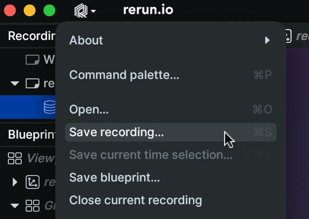
The dataframe SDK loads data from an .RRD file. The first step is thus to save the recording as RRD, which can be done from the Rerun menu:

We can then load the recording in a Python script as follows:
First perform the necessary imports,
from __future__ import annotations

from pathlib import Path

import numpy as np

import rerun as rr
then launch the server to load the recording
server = rr.server.Server(datasets={"tutorial": [example_rrd]})

client = rr.catalog.CatalogClient(server.url())
Query the data
Once we loaded a recording, we can query it to extract some data. Here is how it is done:
dataset = client.get_dataset("tutorial")
df = dataset.filter_contents("/blendshapes/0/jawOpen").reader(index="frame_nr")
A lot is happening here, let's go step by step:
- We first create a view into the recording. The view specifies which content we want to use (in this case the
"/blendshapes/0/jawOpen"entity). The view defines a subset of all the data contained in the recording where each row has a unique value for the index. - In order to perform queries a view must become a dataframe. We use the
reader()call to specify this transformation where we specify our index (timeline) of interest. - The object returned by
reader()is adatafusion.Dataframe.
DataFusion provides a pythonic dataframe interface to your data as well as SQL querying.
Create a Pandas dataframe
Before exploring the data further, let's convert the table to a Pandas dataframe:
pd_df = df.to_pandas()Inspect the dataframe
Let's have a first look at this dataframe:
print(df)Here is the result:
     frame_nr              frame_time  log_tick                   log_time /blendshapes/0/jawOpen:Scalars:scalars
0           0 1970-01-01 00:00:00.000        34 2024-10-13 08:26:46.819571         [0.03306490555405617]
1           1 1970-01-01 00:00:00.040        92 2024-10-13 08:26:46.866358         [0.03812221810221672]
2           2 1970-01-01 00:00:00.080       150 2024-10-13 08:26:46.899699        [0.027743922546505928]
3           3 1970-01-01 00:00:00.120       208 2024-10-13 08:26:46.934704        [0.024137917906045914]
4           4 1970-01-01 00:00:00.160       266 2024-10-13 08:26:46.967762        [0.022867577150464058]
..        ...                     ...       ...                        ...                           ...
409       409 1970-01-01 00:00:16.360     21903 2024-10-13 08:27:01.619732         [0.07283800840377808]
410       410 1970-01-01 00:00:16.400     21961 2024-10-13 08:27:01.656455         [0.07037288695573807]
411       411 1970-01-01 00:00:16.440     22019 2024-10-13 08:27:01.689784         [0.07556036114692688]
412       412 1970-01-01 00:00:16.480     22077 2024-10-13 08:27:01.722971         [0.06996039301156998]
413       413 1970-01-01 00:00:16.520     22135 2024-10-13 08:27:01.757358         [0.07366073131561279]
[414 rows x 5 columns]
We can make several observations from this output:
- The first four columns are timeline columns. These are the various timelines the data is logged to in this recording.
- The last column is named
/blendshapes/0/jawOpen:Scalars:scalars. This is what we call a component column, and it corresponds to the Scalar component logged to the/blendshapes/0/jawOpenentity. - Each row in the
/blendshapes/0/jawOpen:Scalarcolumn consists of a list of (typically one) scalar.
This last point may come as a surprise but is a consequence of Rerun's data model where components are always stored as arrays. This enables, for example, to log an entire point cloud using the Points3D archetype under a single entity and at a single timestamp.
Let's explore this further, recalling that, in our recording, no face was detected at around frame #170:
print(pd_df["/blendshapes/0/jawOpen:Scalars:scalars"][160:180])Here is the result:
160      [0.0397215373814106]
161    [0.037685077637434006]
162      [0.0402931347489357]
163     [0.04329492896795273]
164      [0.0394592322409153]
165    [0.020853394642472267]
166                        []
167                        []
168                        []
169                        []
170                        []
171                        []
172                        []
173                        []
174                        []
175                        []
176                        []
177                        []
178                        []
179                        []
Name: /blendshapes/0/jawOpen:Scalars:scalars, dtype: object
We note that the data contains empty lists when no face is detected. When the blendshapes entities are Cleared, this happens for the corresponding timestamps and all further timestamps until a new value is logged.
While this data representation is in general useful, a flat floating point representation with NaN for missing values is typically more convenient for scalar data. This is achieved using the explode() method:
pd_df["jawOpen"] = pd_df["/blendshapes/0/jawOpen:Scalars:scalars"].explode().astype(float)
print(pd_df["jawOpen"][160:180])
Here is the result:
160    0.039722
161    0.037685
162    0.040293
163    0.043295
164    0.039459
165    0.020853
166         NaN
167         NaN
168         NaN
169         NaN
170         NaN
171         NaN
172         NaN
173         NaN
174         NaN
175         NaN
176         NaN
177         NaN
178         NaN
179         NaN
Name: jawOpen, dtype: float64
This confirms that the newly created "jawOpen" column now contains regular, 64-bit float numbers, and missing values are represented by NaNs.
Note: should you want to filter out the NaNs, you may use the dropna() method.
Next steps
With this, we are ready to analyze the data and log back the result to the Rerun viewer, which is covered in the next section of this guide.