Explore a recording with the dataframe view

In this first part of the guide, we run the face tracking example and explore the data in the viewer.

Create a recording create-a-recording

The first step is to create a recording in the viewer using the face tracking example. Check the face tracking installation instruction for more information on how to run this example.

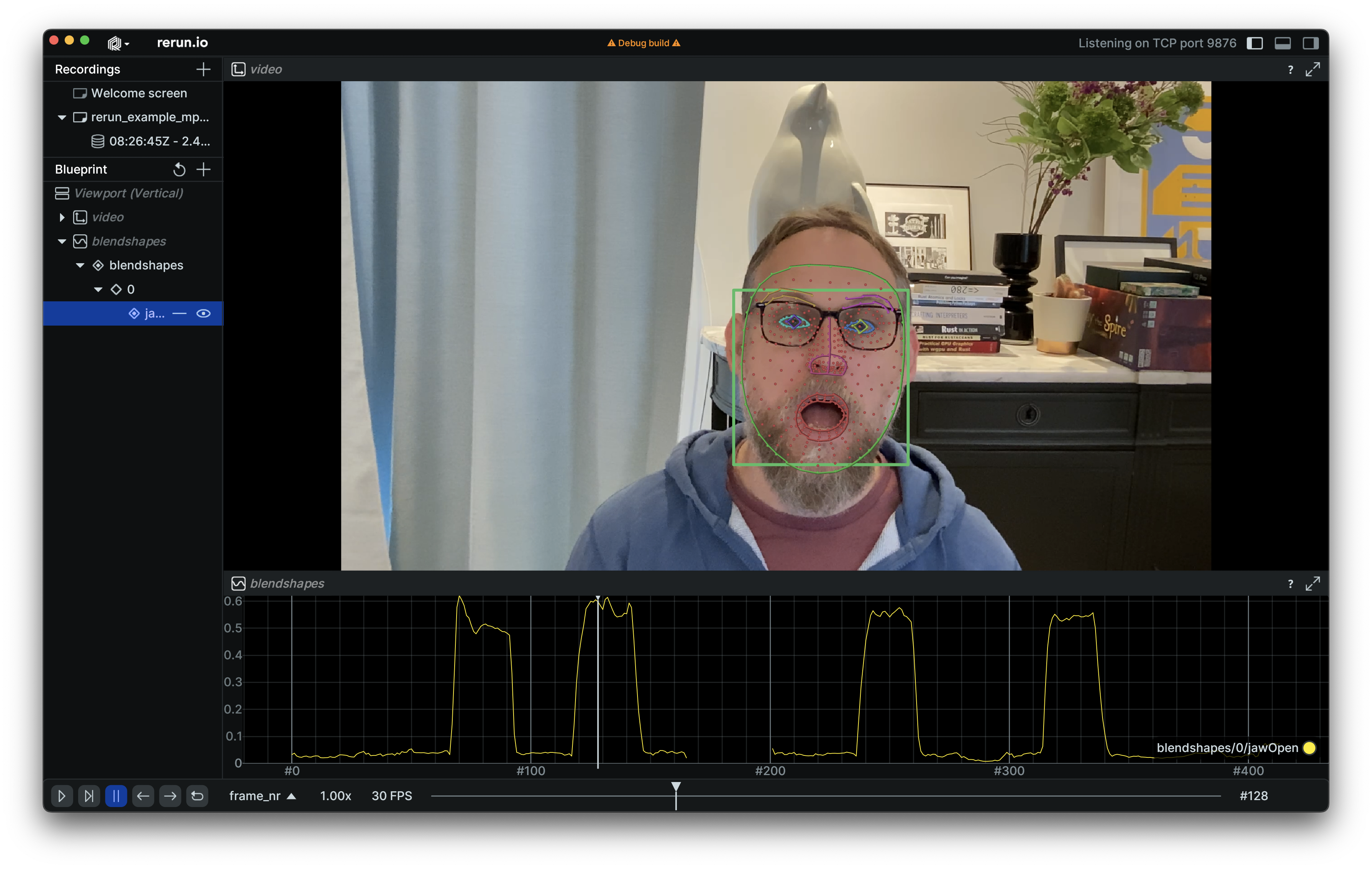
Here is such a recording:

A person's face is visible and being tracked. Their jaws occasionally open and close. In the middle of the recording, the face is also temporarily hidden and no longer tracked.

Explore the data explore-the-data

Amongst other things, the MediaPipe Face Landmark package used by the face tracking example outputs so-called blendshapes signals, which provide information on various aspects of the face expression. These signals are logged under the /blendshapes root entity by the face tracking example.

One signal, jawOpen (logged under the /blendshapes/0/jawOpen entity as a Scalar component), is of particular interest for our purpose. Let's inspect it further using a timeseries view:

This signal indeed seems to jump from approximately 0.0 to 0.5 whenever the jaws are open. We also notice a discontinuity in the middle of the recording. This is due to the blendshapes being Cleared when no face is detected.

Let's create a dataframe view to further inspect the data:

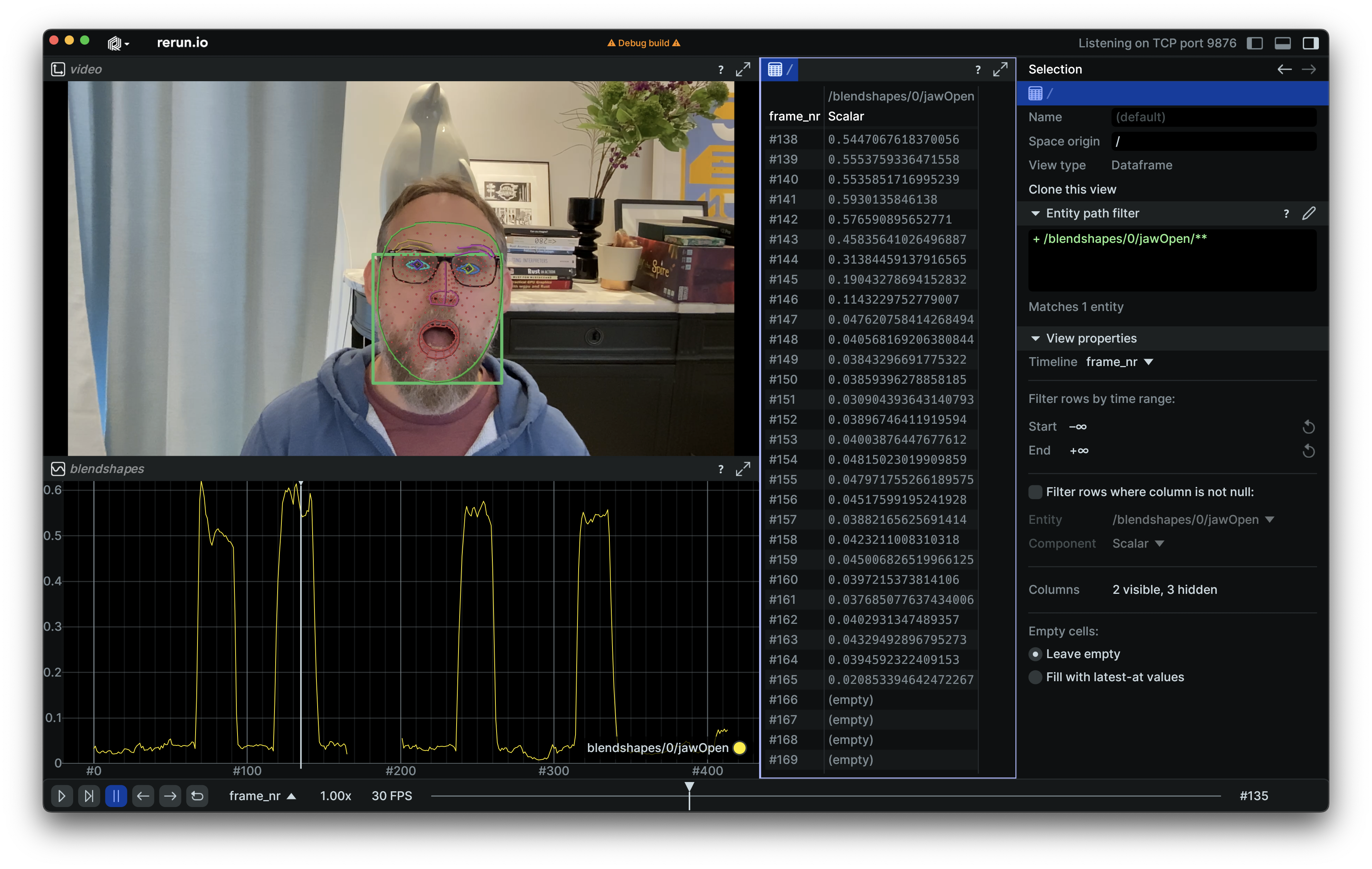
Here is how this view is configured:

• Its content is set to /blendshapes/0/jawOpen. As a result, the table only contains columns pertaining to that entity (along with any timeline(s)). For this entity, a single column exists in the table, corresponding to entity's single component (a Scalar).
• The frame_nr timeline is used as index for the table. This means that the table will contain one row for each distinct value of frame_nr for which data is available.
• The rows can further be filtered by time range. In this case, we keep the default "infinite" boundaries, so no filtering is applied.
• The dataframe view has other advanced features which we are not using here, including filtering rows based on the existence of data for a given column, or filling empty cells with latest-at data.

Now, let's look at the actual data as represented in the above screenshot. At around frame #140, the jaws are open, and, accordingly, the jawOpen signal has values around 0.55. Shortly after, they close again and the signal decreases to below 0.1. Then, the signal becomes empty. This happens in rows corresponding to the period of time when the face cannot be tracked and all the signals are cleared.

Next steps next-steps

Our exploration of the data in the viewer so far provided us with two important pieces of information useful to implement the jaw open detector.

First, we identified that the Scalar value contained in /blendshapes/0/jawOpen contains relevant data. In particular, thresholding this signal with a value of 0.15 should provide us with a closed/opened jaw state binary indicator.

Then, we explored the numerical data in a dataframe view. Importantly, the way we configured this view for our needs informs us on how to query the recording from code such as to obtain the correct output.

From there, our next step is to query the recording and extract the data as a Pandas dataframe in Python. This is covered in the next section of this guide.