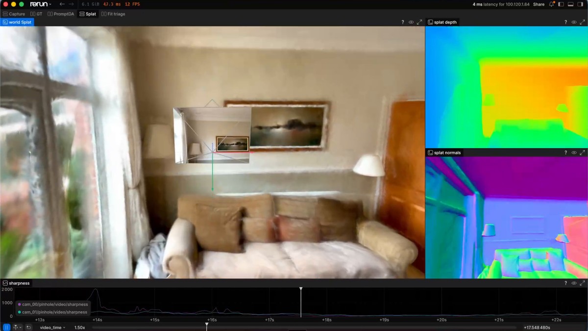
Spotlight: Depth beyond the LiDAR

Written by Pablo Vela 3 days ago

An ultrawide hallway image with a yellow box marking the LiDAR prompt's measured depth coverage, beside LiDAR-aligned MoGe depth. — Left: the camera image, with the phone's depth coverage marked in yellow. Right: MoGe v2 depth after alignment with the LiDAR.

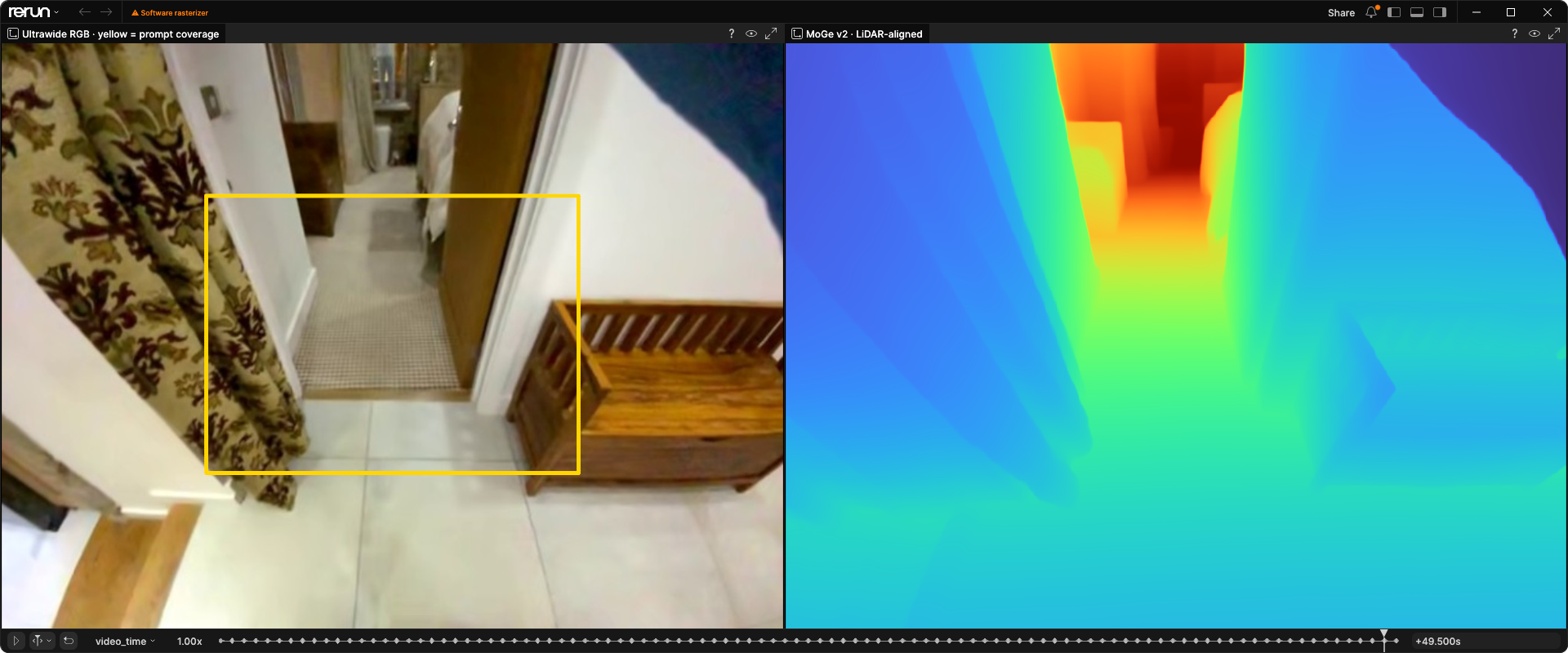
In the first two posts, I ingested ARKitScenes into Rerun and worked on the labels I'd need for training. Now I can actually use them. I want a network that takes the phone's low-resolution LiDAR and an ultrawide image, then predicts detailed depth across that whole image.

Prompt Depth Anything already does this for the wide camera. Extending it to the ultrawide seemed worth trying, especially with training labels now available for that view. I also wanted to keep the work local. I have a 5090 and I wanted to see how far I could get without renting a cluster.

Along the way, I tried replacing the transformer with a much smaller convolutional network. That worked reasonably well on the wide camera and was wicked fast. Training it on the ultrawide was much less successful. I'll show both, along with the MoGe experiment that ended up giving me the depth I needed without another training run.

What changes with the ultrawide?

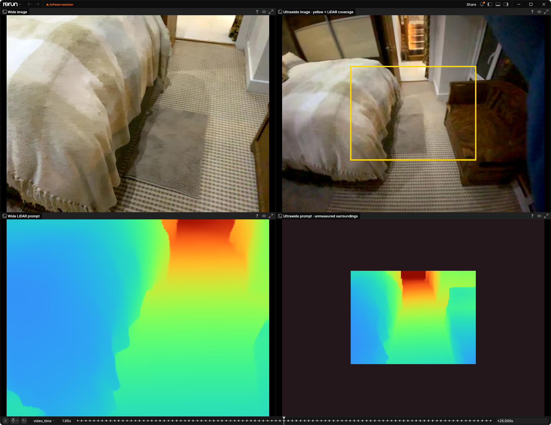
LiDAR covers roughly the wide camera's view, but only the middle of the ultrawide. The model has to predict depth beyond that measured area too. Part 2 covers the camera geometry and how I built labels for the ultrawide.

Rerun capture of the same bedroom: wide and ultrawide camera images above their LiDAR prompts. The wide prompt fills its view, while the ultrawide prompt occupies only a small central rectangle matching the yellow box above. — Actual training inputs from the same recording and timestamp, shown in Rerun. Images above, depth prompts below. On the ultrawide, the LiDAR covers just under a quarter of the image; the dark area around the prompt is missing depth, not a surface at zero meters.

Training Prompt ZipDepth on the wide camera

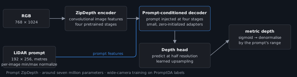
I didn't start by training the transformer. Repeated runs on a large model would take longer, and I was interested in whether a small CNN could do enough of the job. That's where ZipDepth came in. It's a convolutional depth model trained with distillation from Depth Anything V2, so it was a reasonable starting point for a smaller prompted model. PromptDA has a Depth Anything V2 backbone, so I thought using ZipDepth would be a cool experiment, and from what I saw it was really fast to train and run.

I took the released ZipDepth weights and added adapters to feed the LiDAR prompt into its decoder. The resulting model has around seven million parameters. I've called it Prompt ZipDepth here, though you'll find it as ZipDepth-PromptDA in the code and some of the viewer captures.

Prompt ZipDepth architecture, with RGB passing through the pretrained convolutional encoder and the normalized LiDAR prompt injected at four decoder stages. — The image goes through the pretrained ZipDepth encoder. The LiDAR prompt enters at four decoder stages, with the final prediction converted back to meters. Dimensions are height × width.

Before adding the ultrawide, I wanted to check that this was better than just resizing the wide-camera LiDAR with bilinear interpolation.

For training, I used the PromptDA predictions already stored in the catalog, about a million frames across roughly two thousand ARKitScenes recordings. Each sample paired one of those predictions with its RGB, LiDAR, and confidence map. I kept a small set of complete recordings out of training for evaluation.

The connection starts with Rerun's CatalogClient(...).get_dataset(...). The catalog helper then selects recordings with a promptda layer and reads their orientation metadata. I split those recording IDs before loading any training frames:

catalog: PromptDACatalog = load_promptda_catalog(
    config.catalog_url, config.dataset_name,
)
split: tuple[list[str], list[str]] = split_holdout_segments(
    catalog.segment_ids, config.holdout_count, config.holdout_seed,
)
train_ids: list[str] = split[0]
holdout_ids: list[str] = split[1]

The snippets here are shortened excerpts from the experiment code, using its existing configuration and setup. They're meant to show the pieces; the linked files contain the imports and full implementations.

One thing to consider here, I never had to convert the on disk RRD files to a different format such as parquet or webdataset. The rerun catalog model took care of getting things into the right format so you can just directly create a pytorch dataloader.

The streaming dataset does that work in producer threads. Each producer gets its own decoder and sample builder; the builder handles orientation, resizing, augmentation, and conversion of depth to meters. PyTorch only needs to batch the prepared samples:

dataset: CatalogPromptDepthDataset = CatalogPromptDepthDataset(
    catalog.dataset_entry, train_ids, catalog.row_by_id,
    device=device,
    builder_factory=builder_factory,
    num_producers=config.num_producers,
    load_confidence=False,
)
loader: DataLoader[dict[str, Tensor]] = DataLoader(
    dataset, batch_size=config.batch_size,
    num_workers=0, pin_memory=False, drop_last=True,
)

Here, builder_factory creates a CudaSampleBuilder with metric targets. num_workers=0 is deliberate: CUDA decoding stays in the training process, with the producer threads supplying concurrency. The tuned training path also skips fetching confidence, since the student takes the raw LiDAR prompt and checks its depth range internally. Evaluation still uses confidence for its diagnostics.

Even then, the first run only saw about half a pass through the dataset. I trained for much longer before settling on the reference model used below, with several passes' worth of samples by the end.

The training step is fairly ordinary once a batch is ready. RGB is converted to floating point in [0, 1]; prompt and target depths are already in meters. With those tensors on the GPU, the BF16 update is:

with torch.amp.autocast("cuda", dtype=torch.bfloat16):
    pred: Float[Tensor, "b 1 h w"] = student(images, prompt_depth)
    loss: Float[Tensor, ""] = criterion(
        pred=pred, target=target_depth, mask=target_valid,
    )[0]

loss.backward()
torch.nn.utils.clip_grad_norm_(student.parameters(), max_norm=1.0)
optimizer.step()
scheduler.step()
optimizer.zero_grad(set_to_none=True)

The metric loss combines masked L1 depth error with a multi-scale gradient term. Missing target pixels are excluded. Checkpointing and TensorBoard logging sit around this loop.

Better than upsampling, but still missing detail

With a trained model in hand, I wanted to see how it performed compared to naive upsampling. This bookshelf example in a data sample the network never saw is a good place to see what the model learned. Bilinear upsampling blurs the shelf edges and side panel into the surrounding surfaces. Prompt ZipDepth separates them much more clearly.

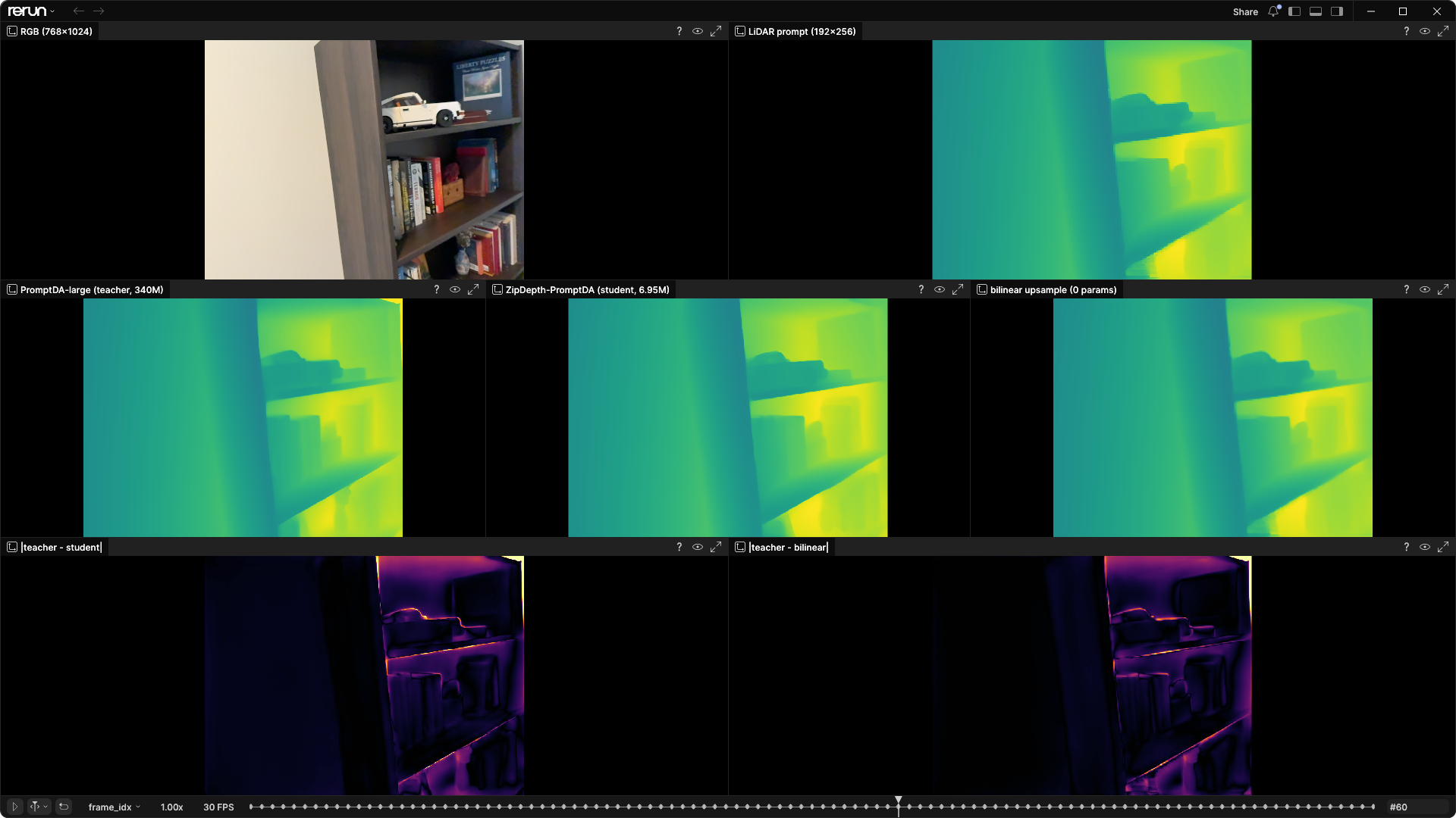
A real Rerun comparison of a bookshelf: RGB and LiDAR, PromptDA teacher, Prompt ZipDepth student, bilinear baseline, and teacher-relative disagreement maps. — This Polycam capture is separate from the training data. Compare the shelf edges and side panel in the student and bilinear views. The bottom maps show where they disagree with the PromptDA teacher.

Across the wide-camera holdout, the student roughly halved the edge error of validity-aware bilinear upsampling, from around fourteen centimeters to seven. I measured this at the strongest depth gradients in the PromptDA labels. That measures how closely the student matches its teacher, not how close either model is to a laser scan.

The plant was harder. PromptDA picks out individual leaves that my model merges together, even though both get the same image and LiDAR prompt.

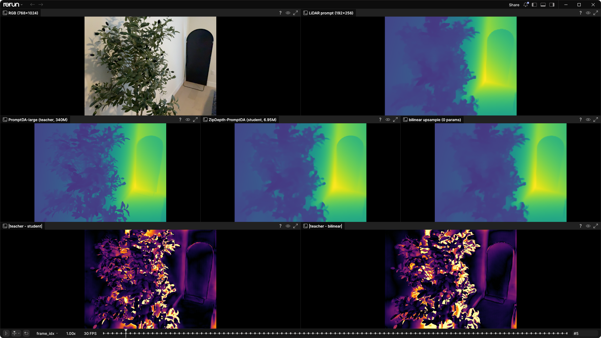
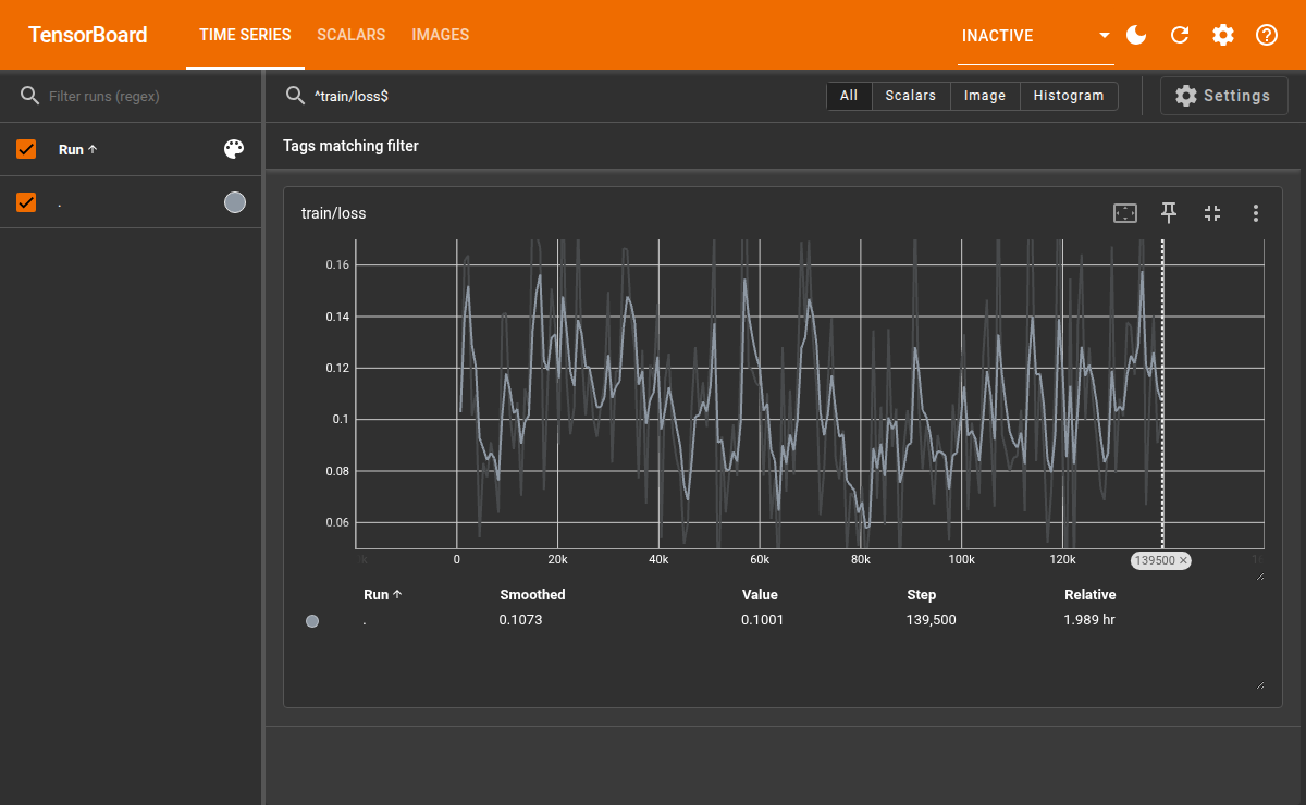
A leafy plant in the Rerun comparison. PromptDA separates individual leaves, while the student merges many of them into a smoother surface. — A difficult frame from the Polycam capture. The teacher preserves the leaf shapes; the student produces a much smoother blob.

I spent a fair amount of the training work on this: longer runs, stronger gradient losses, and changes to the decoder and upsampling head. The leaves never got a reliable fix. A few changes even improved the ARKitScenes score while making this Polycam example worse, which is why I kept checking the actual predictions in Rerun.

Some of the problems were in my setup. RGB and depth resizing disagreed about pixel centers, leaving the inputs and labels slightly misaligned. Batch-normalization behavior also interfered with the early learning-rate comparisons. I had to sort those out before I could trust the results.

After those fixes, a higher learning rate reached roughly the same early quality in half an hour instead of an hour and a half. That was useful for trying changes, although the short runs still didn't match the longer-trained reference model.

What does it look like in 3D?

Since the point of all this is reconstruction, here's the same Polycam capture fused three ways: with raw phone depth, PromptDA, and Prompt ZipDepth.

Left to right: raw LiDAR, PromptDA, and Prompt ZipDepth, using the same recorded poses and TSDF fusion settings. The bottom row shows the RGB and depth maps as they arrive.

All three recover the broad shape of the room. Keeping the source depth below each mesh helps separate the network's output from what happens during fusion. Holes and rough surfaces can also come from the poses or voxel resolution, so this isn't a clean measure of depth accuracy on its own.

How fast is it?

The speed is the reason I'm still interested in this model. In my TensorRT benchmark, Prompt ZipDepth was roughly thirty times faster than the teacher: well under a millisecond per frame, compared with around twenty milliseconds.

Those timings are from the 5090 using FP16, batches of eight, and similar image sizes. I divided the network's batch execution time by eight; decoding and reconstruction aren't included. The video above uses a different student backend, so its playback isn't a demonstration of that benchmark. I'd like to use a model this small on-device, but I haven't benchmarked it on a phone.

For now, being able to train and check an idea quickly was enough reason to try the ultrawide version.

Try it on Hugging Face

I ported the comparison to a Hugging Face Space so you can try it without setting anything up locally. Run the bundled Polycam capture to compare raw LiDAR, PromptDA, and Prompt ZipDepth in Rerun, inspect the depth maps and 3D reconstructions, and see the per-model timings and speedup in the Outputs panel.

The Space runs both models in eager PyTorch on ZeroGPU, so its timings will differ from the TensorRT benchmark above. For a shorter run, open Debug and use Quick check: 1 frame. That includes cold-start overhead; use the full capture for a more useful speed comparison. Runs depend on the available ZeroGPU quota.

Now give it the ultrawide image

This is where the post-processing from Part 2 comes in. I fused the wide-camera PromptDA predictions into a mesh, then rendered depth from each ultrawide camera pose. These runs used the TSDF-rendered labels, rather than the Gaussian-splat labels also explored in that post. The rendered depth covers surfaces seen during the capture that lie outside a single frame's LiDAR prompt.

That gave me around a million and a half ultrawide frames with labels. I rectified the images and placed the wide LiDAR in the middle of the prompt, leaving the rest marked as missing. The recorded images are only 640×480 in landscape, or 480×640 in portrait, so there's less RGB detail available here than in the wide-camera runs, even after resizing for the network.

In the ultrawide experiment's zipdepth.catalog.ultrawide helpers, that placement looks like this. lidar_depth_m is the orientation-corrected LiDAR map in meters:

placement: PromptPlacement = prompt_placement(
    DEFAULT_ULTRAWIDE_PROMPT_SCALE,
)
block: Float32[Tensor, "block_h block_w"] = resize_prompt_block(
    lidar_depth_m, placement,
)
prompt: Float32[Tensor, "192 256"] = pad_prompt_block(
    block, placement,
)

The resize uses nearest-exact sampling, so it doesn't blend neighboring depth readings. The padding is zero, which the model treats as missing input, not a surface at zero meters.

I resumed from the wide-camera checkpoint with an even mix of wide and ultrawide samples. I wanted to keep the wide-camera quality while learning the new view. The first run took a couple of hours.

An enlarged TensorBoard loss chart from the first ultrawide training run, in dark mode. — Training loss for the first ultrawide run in TensorBoard, with smoothing enabled. The curve stays noisy, so I also checked the held-out predictions below.

Here's what that model produced on a recording it hadn't trained on.

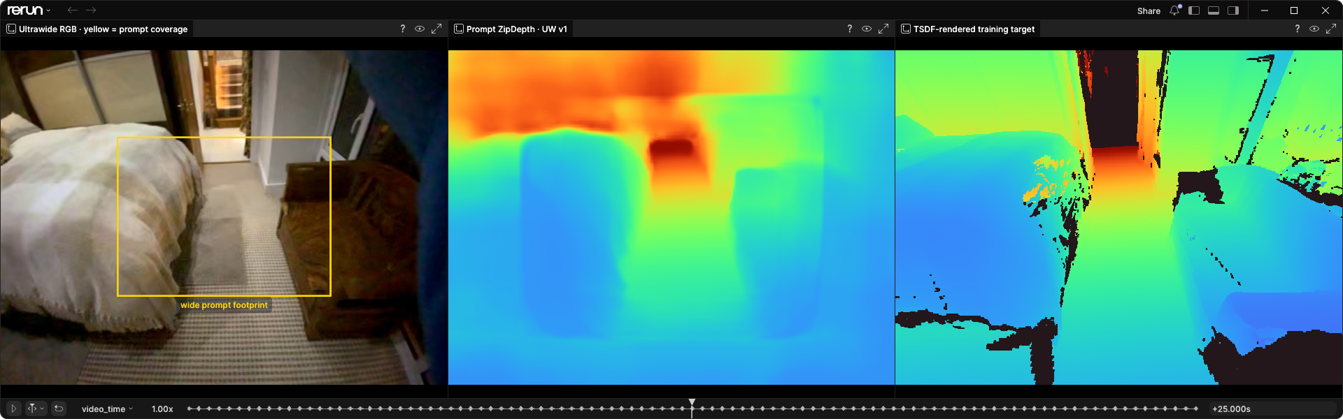
The ultrawide bedroom image with its central prompt footprint, the trained ultrawide student's smooth and distorted prediction, and the TSDF-rendered target. — The first ultrawide model on a held-out recording. It loses the doorway and merges surfaces outside the prompt. The MoGe comparison below uses this same frame and depth scale. Black regions in the target are missing mesh coverage, not measured empty space.

The doorway is mostly gone, and surfaces outside the prompt run into each other. This was better than applying the wide-only model unchanged, including on the holdout score, but I wouldn't use it for the reconstruction I wanted. Wide-camera quality had also slipped despite the mixed training data. For me, this attempt had failed.

Why the ultrawide attempt fell short

My main suspicion is that the network was simply too small. It already struggled with fine detail on the wide camera, and now I was asking it to predict depth across most of an image without any LiDAR measurements there. The larger PromptDA model might handle this better, but I haven't trained it on the ultrawide task. It's quite possible that it would struggle too.

There were also problems in the setup. One was how I converted the network's output back to meters, using the minimum and maximum depth in the prompt as the output range. On the wide camera, that's a useful constraint. On the ultrawide, a wall outside the prompt can be farther away than anything the LiDAR measured, and the model has no way to output its depth.

That wasn't a rare case: roughly a quarter of the valid target pixels outside the prompt were also outside its depth range.

I tried a second version that could use the full 0.1–4 m training range when prompt coverage was low, along with stricter filtering of the targets. Unfortunately, error outside the prompt got worse and wide-camera quality slipped further. Removing the range restriction wasn't enough.

The rendered labels also have holes and imperfect edges, and the model was trying to learn the new task without losing the old one. I didn't isolate those effects from model size, so the small-network explanation is still my best guess rather than something these runs prove.

This was still the kind of experiment I wanted to be able to do locally. A couple of hours was enough to get a result I could inspect and decide what to try next.

What if I just align MoGe to the prompt?

At this point, I could have gone back to PromptDA and trained the larger transformer for the ultrawide task. Before committing to that, I wanted to try something much simpler.

MoGe v2 already produces sharp, detailed geometry from an image. I also had a metric depth prompt sitting in the middle of that image. Could I just align the two and use MoGe's depth?

The implementation was:

Run MoGe on the rectified ultrawide image.
Compare its depth with valid LiDAR measurements inside the central footprint.
Take the median LiDAR-to-MoGe depth ratio as a scale factor.
Apply that factor to the full MoGe depth map, including the unprompted surroundings.

This uses the pretrained MoGe model as-is. The only thing I fit is one scale factor per frame.

The core calculation is just a median ratio. Here, moge_on_prompt has been resampled onto the LiDAR grid, and paired selects cells inside the footprint where both depths are valid:

ratios: Float32[Tensor, "n"] = (
    lidar_depth_m[paired] / moge_on_prompt[paired]
)
scale: float = float(torch.median(ratios))
aligned_depth: Float32[Tensor, "h w"] = moge_depth * scale

The full implementation checks that enough valid pairs remain and falls back to a scale of one if the fit can't be used. The same factor scales the high-resolution MoGe output, including everything outside the prompt.

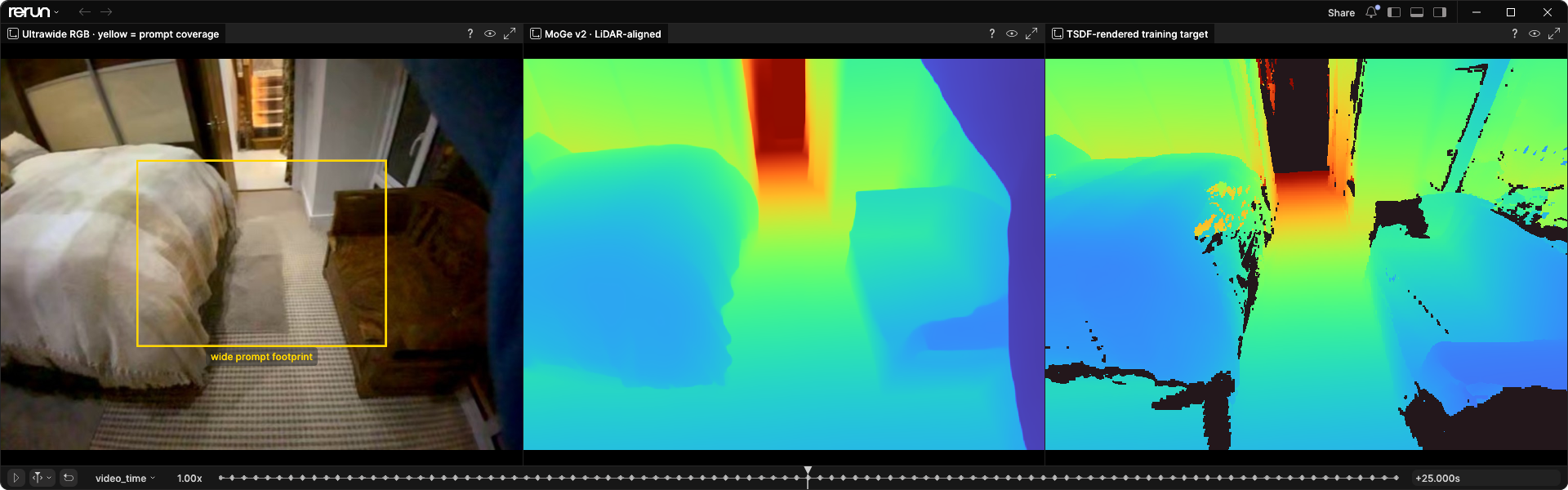
The same ultrawide bedroom at the same timestamp, now with aligned MoGe depth beside the rendered target. — Same frame as the failed ultrawide prediction above. Aligned MoGe keeps the doorway, bed, and chair much more distinct. This view shows MoGe itself after LiDAR alignment, not a prompted student fed with MoGe predictions.

This was much closer to what I wanted. The doorway, bed, and chair stay separate, including outside the measured part of the image.

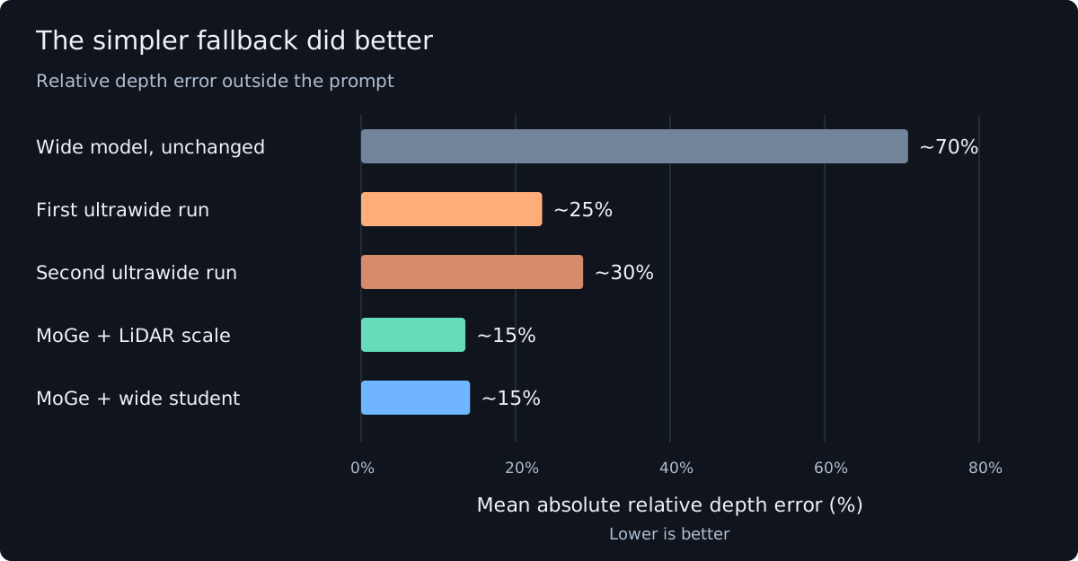
Peripheral depth error on the same ultrawide holdout, comparing the wide-only student, two ultrawide training runs, aligned MoGe, and a MoGe-filled student. — Mean per-frame relative depth error outside the prompt, shown as a percentage. Lower is better. Bar lengths use the measured values; labels are rounded for readability. All methods use the same roughly fifteen hundred frames from twenty held-out recordings, scored against TSDF-rendered targets rather than independent ground truth.

It also had lower error against the rendered labels than either ultrawide-trained student on the same held-out recordings.

I tried a couple of variations. One filled the missing prompt area with aligned MoGe depth and passed it through the wide-camera student, but the extra network didn't improve the result. Fitting a scale and a shift also did worse outside the prompt than fitting scale alone. So I kept the scale-only MoGe output.

Aligned MoGe over the capture, with the measured prompt footprint marked in yellow. Playback is accelerated. Each frame is predicted and aligned independently; this clip is a visual check, not a temporal-consistency benchmark.

Of course, MoGe is a large transformer too. I've given up the small model's inference speed, even though I avoided training another model. Each frame is also predicted and aligned independently. I haven't measured how stable that is over time, and a method that uses the sequence could do better. For the ultrawide depth I need right now, though, this looks good enough to keep working with.

Where this leaves the project

I still like Prompt ZipDepth for the wide camera. It improves on plain upsampling, runs very quickly, and gave me a way to try training ideas on the hardware I already have. The transformer keeps more detail, especially on things like the plant, so which one I'd use depends on how much quality I can give up for speed.

The ultrawide version isn't something I'd use yet. For that part of the pipeline, I'm going with aligned MoGe for now. It's a different answer from the model I expected to train, but it gives me a useful depth map and lets me move on with the reconstruction work.

Having the inputs, labels, and predictions together in Rerun made these runs much easier to compare. I could check the same frame across models, then see what its depth did to the reconstruction. That's what the data work in Parts 1 and 2 was for, and it's what I'll keep using as the models change.

Could diffusion be a better fit?

Another model I'd like to try is Marigold V2. It adapts a pretrained image-generation and editing model for depth prediction, and the authors also show metric depth completion. That seems closer to what I need: use the image to fill in depth where the LiDAR has no measurements. My small CNN was a quick experiment, and I'm glad I tried it, but I suspect this is a better direction for the ultrawide problem. I haven't tested it on these captures yet.

The tradeoff is that theres no chance this runs in realtime on mobile hardware. Marigold V2 predicts depth in a single step, but it still uses a large diffusion transformer. The released implementation needs well over ten gigabytes of GPU memory for a roughly megapixel image, even with quantization. I'd expect it to be much slower than Prompt ZipDepth, though I haven't timed it. In its current form, I'd treat it as an offline reconstruction option, not something I'd expect to run in real time on a phone.

References

Part 1: The data layer and Part 2: Better labels.
Prompt Depth Anything and its paper.
ZipDepth, the pretrained convolutional depth model.
MoGe, including MoGe v2 and the released inference code.
Marigold V2, a possible next experiment with diffusion-based depth completion.
Depth-training package and Polycam trio viewer. The ultrawide results described here come from the saved experiment branches, not a claim that every experiment has landed on main.

I reused these holdout recordings while developing the models. The split is by recording, and I haven't verified that rooms are separate across the split. Treat the scores as comparisons for this project, not as a final test of performance on new rooms.