Spotlight: Better labels for 3D reconstruction
In the previous blog, we laid out the path for building a system that takes as input iPhone sensor data and produces metrically accurate 3D data. This is to make it possible to use human demonstration data as input for robot training, an important new scaling axis that the industry is currently tapping into.
This involved setting up the data pipeline for our dataset of choice, ARKitScenes, a dataset from Apple for 3D reconstruction and semantic understanding from just a single iOS device. We converted this dataset into the Rerun data format (rrd) so that visualizing, querying, and training are all accessible from a single easy-to-use dataset.
In this blog, we'll dig into the labels that ARKitScenes provides, the problems found in those labels, and how we'll address them using post-processing to generate a higher-fidelity pseudo ground truth without modifying the original data and instead registering it as layers on top with Rerun!
Why the existing labels are not enough for training
The data
Before training anything, we need to inspect the registered data and understand where it fails. We cannot curate what we have not looked at, and the streams below are what a dataloader will actually see.
Here is everything one scan carries, all of it on a single timeline.
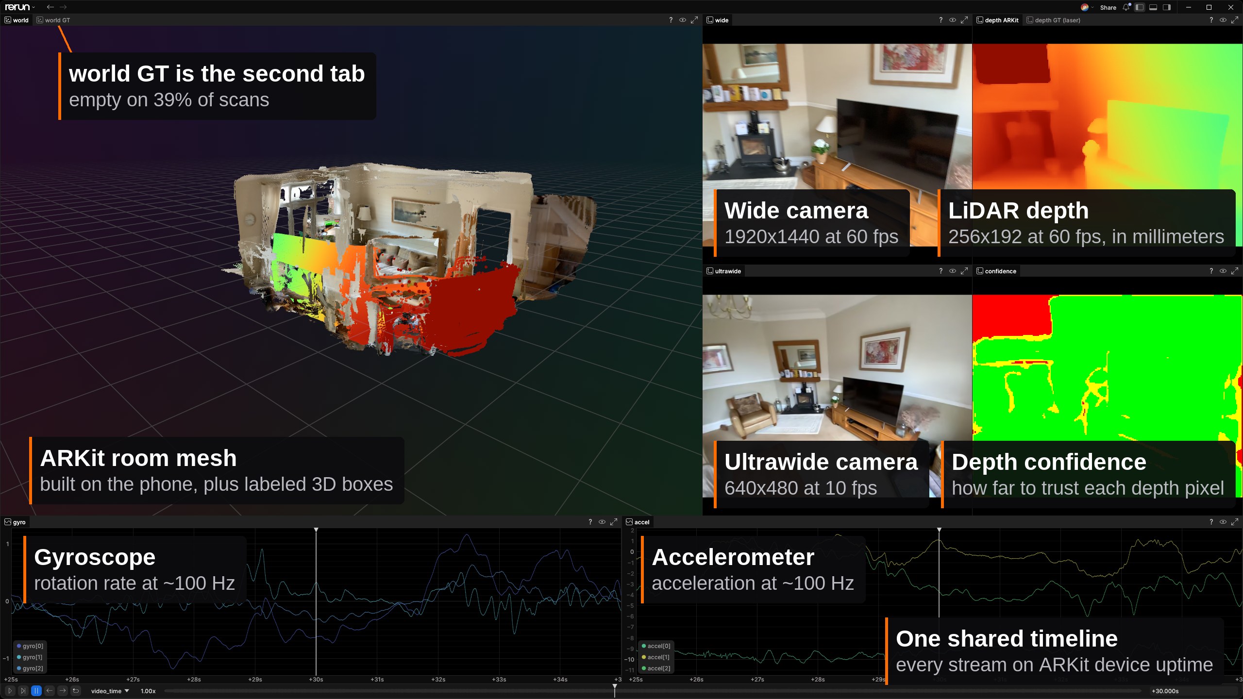
| Data | What it is | Shape and rate | Coverage |
|---|---|---|---|
| Wide video | Color from the main camera | 1920×1440 at 60 fps | Every scan |
| Ultrawide video | Color from the wide field of view camera | 640×480 at 10 fps | Every scan |
| ARKit LiDAR depth | Depth measured by the phone, in millimeters | 256×192 at 60 fps | Every scan |
| Depth confidence | How far to trust each ARKit LiDAR pixel | 256×192 at 60 fps | Every scan |
| Camera poses | Where the device was, from ARKit's VIO | 60 Hz | Every scan |
| Calibration | Intrinsics per frame, and a 1.2 cm baseline | Per frame | Every scan |
| Accelerometer | Acceleration | ~100 Hz | Every scan |
| Gyroscope | Rotation rate | ~100 Hz | Every scan |
| Device attitude | Fused orientation from CoreMotion | ~100 Hz | Every scan |
| ARKit mesh | The room mesh ARKit built on the device | Static | Every scan |
| 3D boxes | Labeled oriented boxes around objects | Static | Every scan |
| Laser trajectory | Poses registered against the laser scan | Per frame | Some scans |
| Laser depth | Depth rendered from the stationary laser scan | Per frame | Some scans |
The primary source of ground truth for this dataset (in the context of pose and depth estimation) comes from the FARO laser scanners. But as with any real data, there are some issues that arise.
Digging through the dataset we find the following
- Many segments are missing laser scans
- Even when laser scans are available they often have lots of occlusions and holes
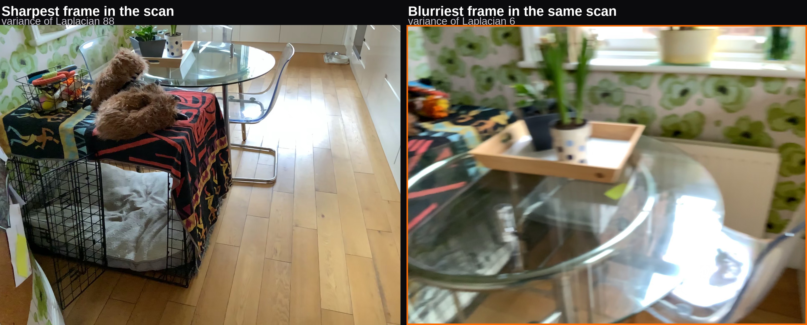
- The actual video from the iOS device often has motion blur
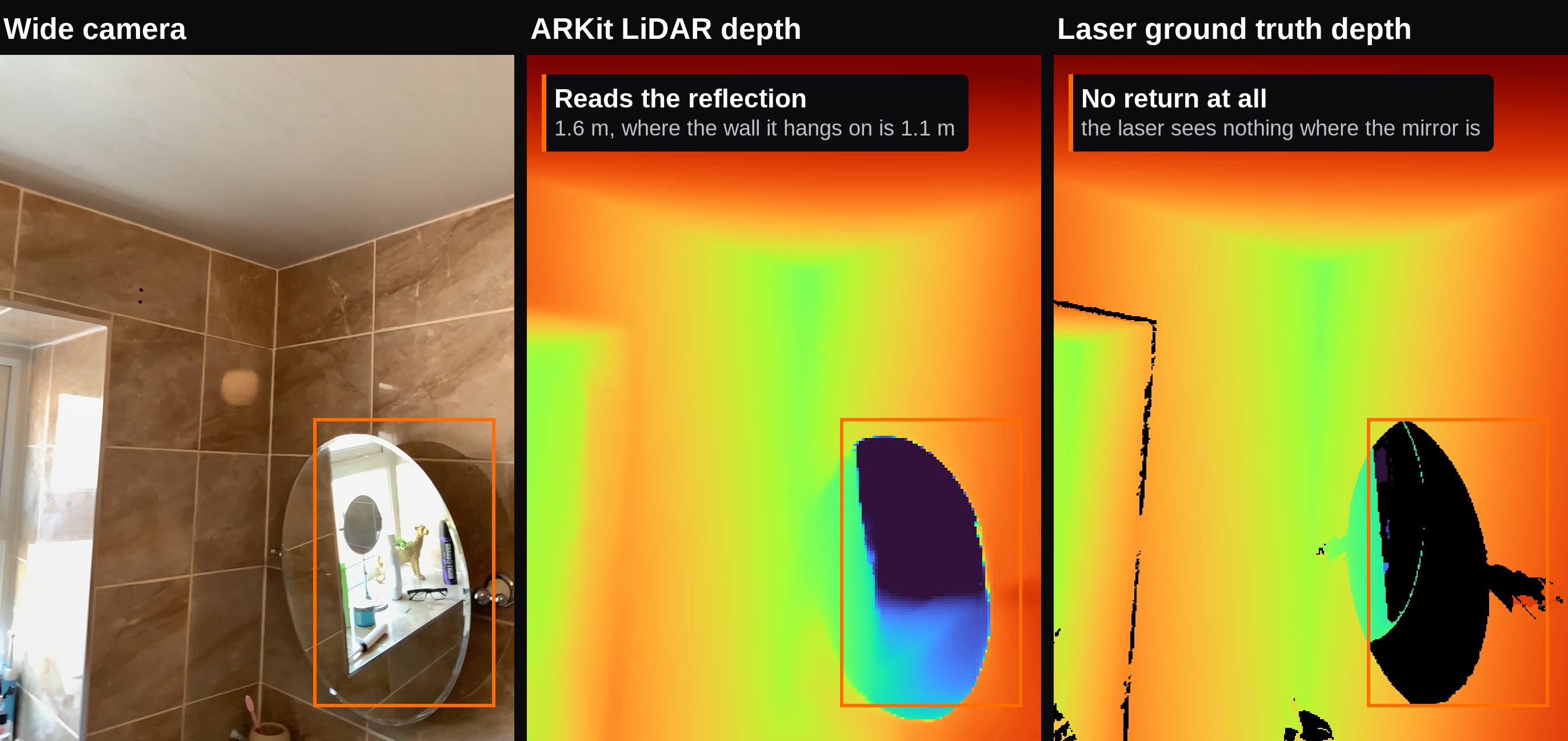
- Transparent and reflective surfaces cause problems for both the laser scan and the iOS lidar scan
The laser is still the best available reference where it has a valid return, but it cannot serve as the only training label. Let's walk through each of the issues below.
Missing laser scans
Not all captures have reference scans from the Faro Focus S70 stationary laser scanner. Of the 5,071 captures in the raw release, only 3,068 have released laser point clouds, covering 1,004 of the 1,664 venues. The other 2,003 captures have none. For those scans, the available inputs are the paired wide and ultrawide videos, ARKit VIO poses, IMU values, and extremely low-resolution, noisy 256×192 phone depth. Any training recipe that requires laser labels writes off those scans, along with future captures for which a Faro scan will never exist.
Occlusions and holes
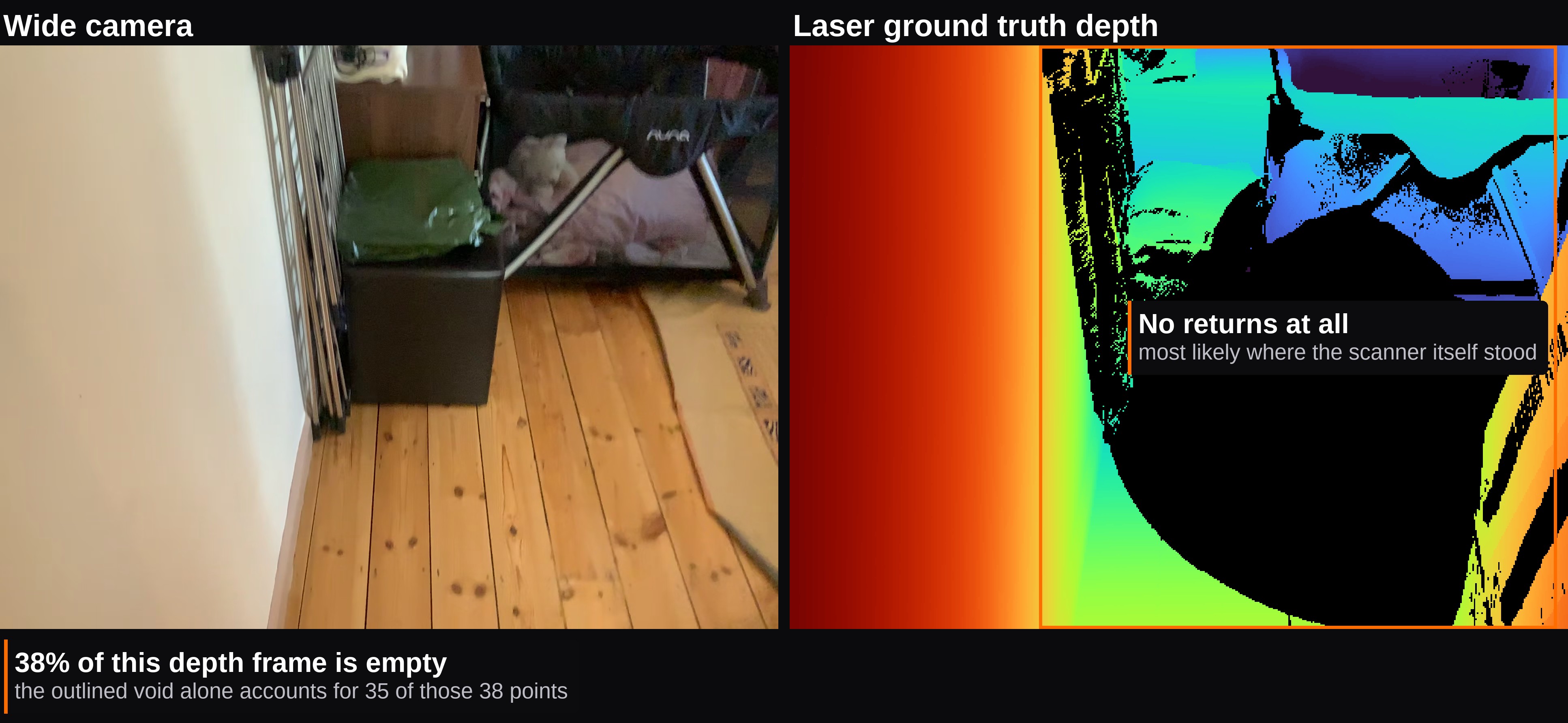
A stationary scanner cannot see behind occluders or beneath its own tripod position. Several scan positions therefore produce incomplete meshes, depth maps with large holes, and poor edges.
Motion blur and camera instability
Unsteady filming causes edge deformation, ghosting, and smeared textures. Those frames can corrupt the reconstruction used to make labels, then teach a model from the corrupted result. Sharpness is therefore a label-quality signal, not just an image-quality preference.
Transparent and reflective objects
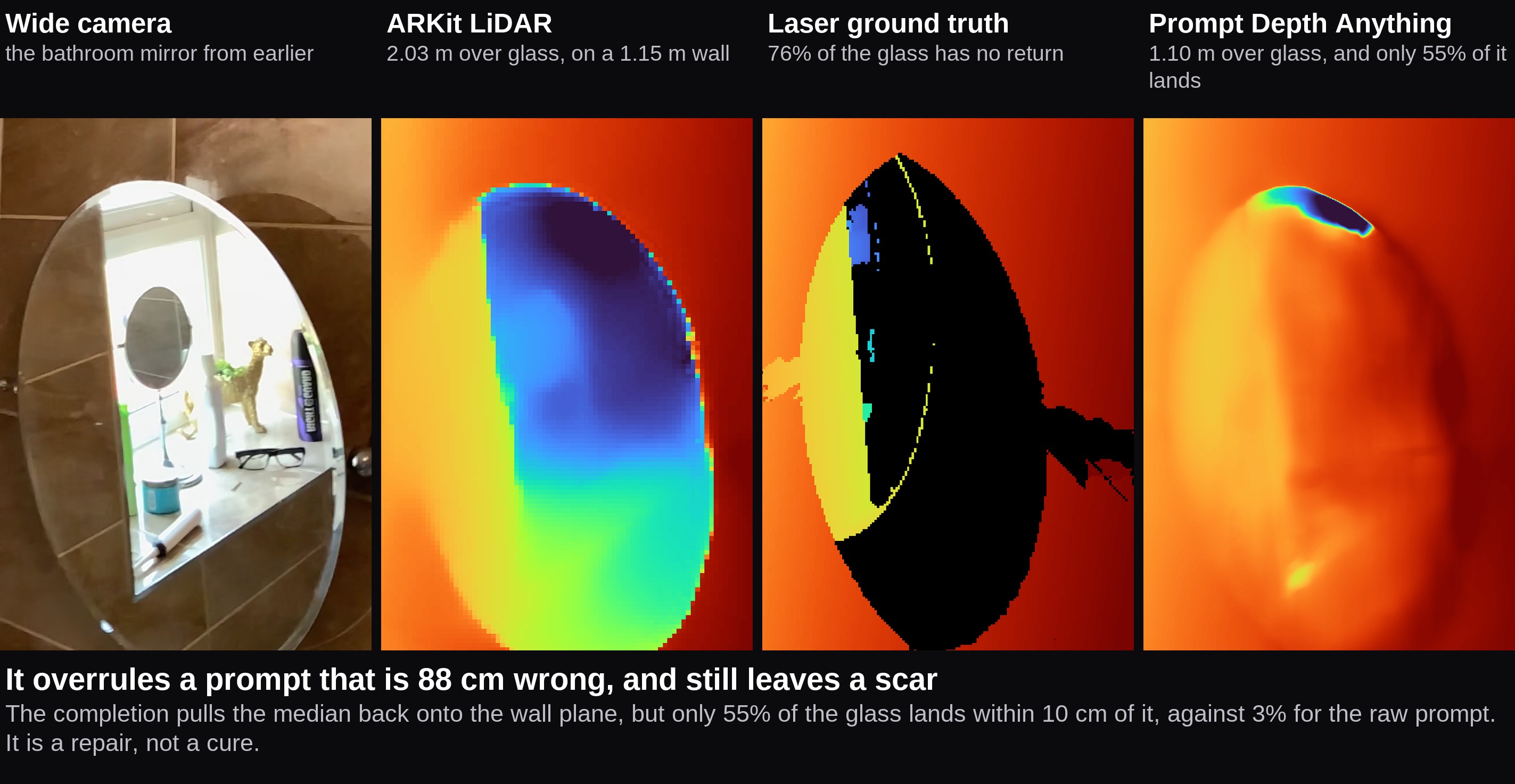
Televisions, mirrors, and windows cause different failures in both the stationary laser scanner and the iPhone's time-of-flight sensor. A missing return and a confident return from a reflected room require different handling, even when both look wrong in the resulting depth map.
Building a candidate pseudo-label layer
The laser depth is missing at the start and end of most scans, drops out wherever registration fails, and for many scans never existed at all. We need a candidate label that can be produced from every phone capture, while reserving valid laser returns as an independent referee.
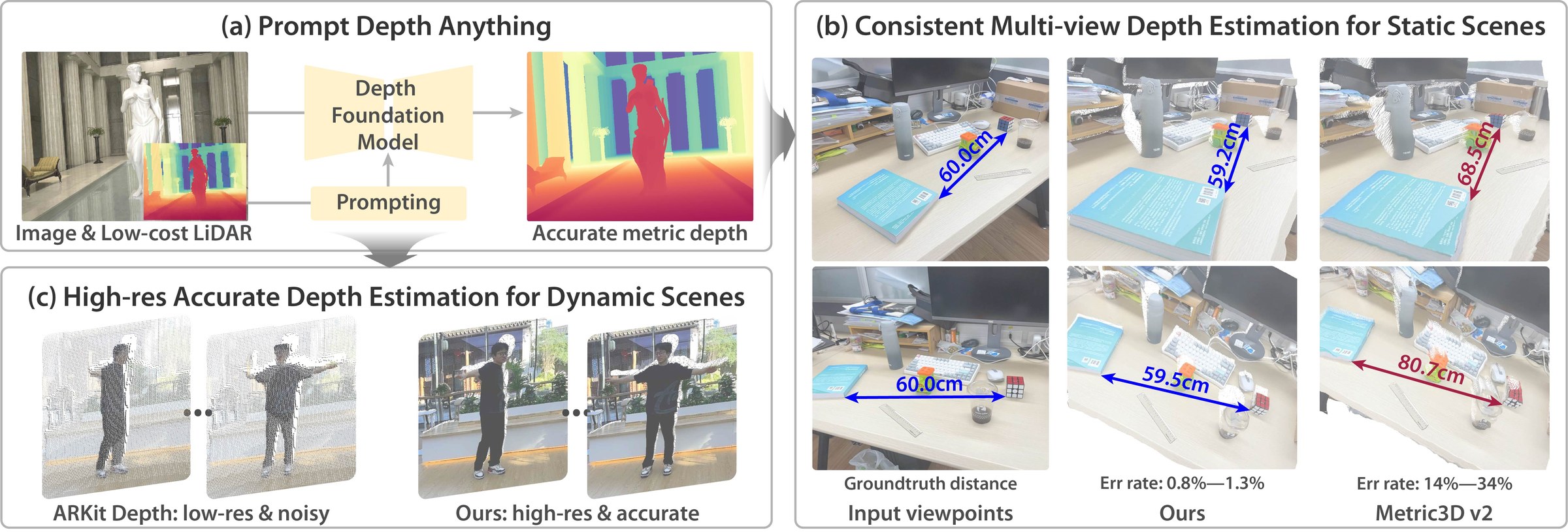
The starting point comes from the Prompt Depth Anything paper, which encountered the same problem on ScanNet++. Its laser labels had holes and soft edges, so the authors trained one Zip-NeRF per scene, rendered depth from that reconstruction, and used the laser for absolute values while using the reconstruction for gradients.
We start with the open Prompt Depth Anything model, or PromptDA, instead of fitting a Zip-NeRF per scene. PromptDA takes a wide RGB frame and the phone's own 256×192 LiDAR depth as a prompt, then predicts dense metric depth at 1008×756. The phone provides those inputs for every scan, including those with no laser reference. This makes PromptDA a useful first candidate, it extends coverage while leaving the laser free to test accuracy where the laser is reliable.
PromptDA still predicts one frame at a time, with nothing tying its frames together. So we keep the second half of the paper's recipe, fitting a reconstruction and rendering labels out of it, but we fit a Gaussian splat instead of a Zip-NeRF. This mostly comes down to how computationally expensive it is to train. Zip-NeRF costs roughly 20 GPU-hours per scene, and running PromptDA across a 60 fps scan means paying for tens of thousands of frames. A splat needs only a few hundred sharp views, and once fit, it renders depth cheaply for the full sequence and from any pose, including the ultrawide camera that has no LiDAR prompt of its own.
The following three cases test where the candidate helps and where it still fails.
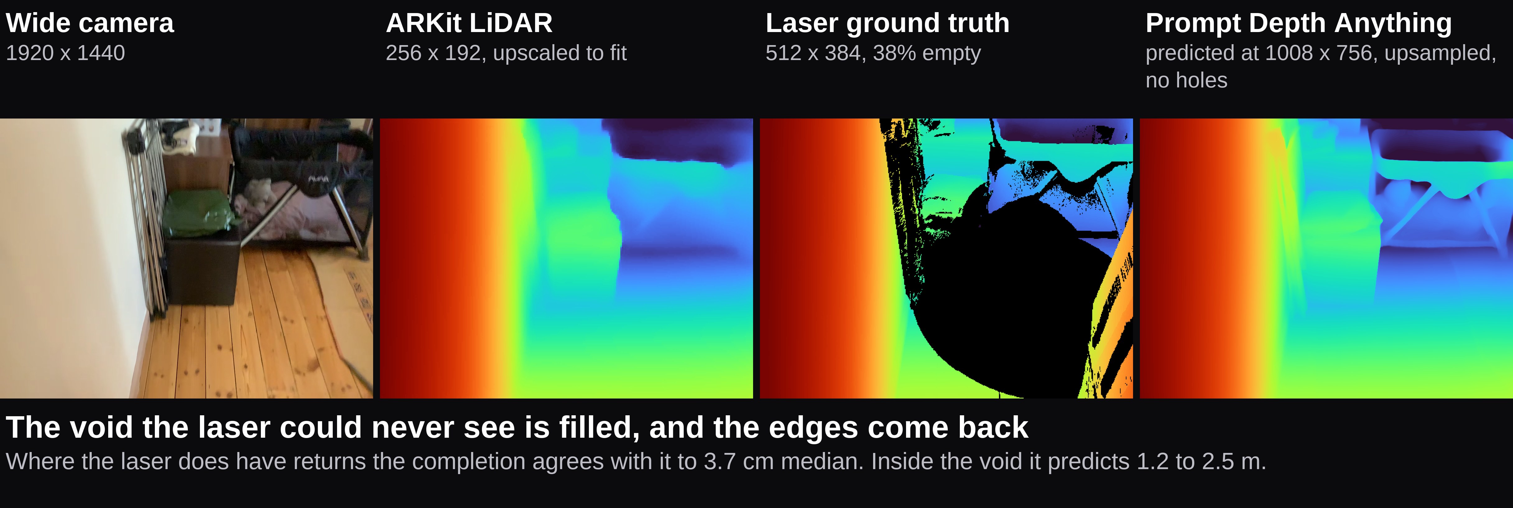
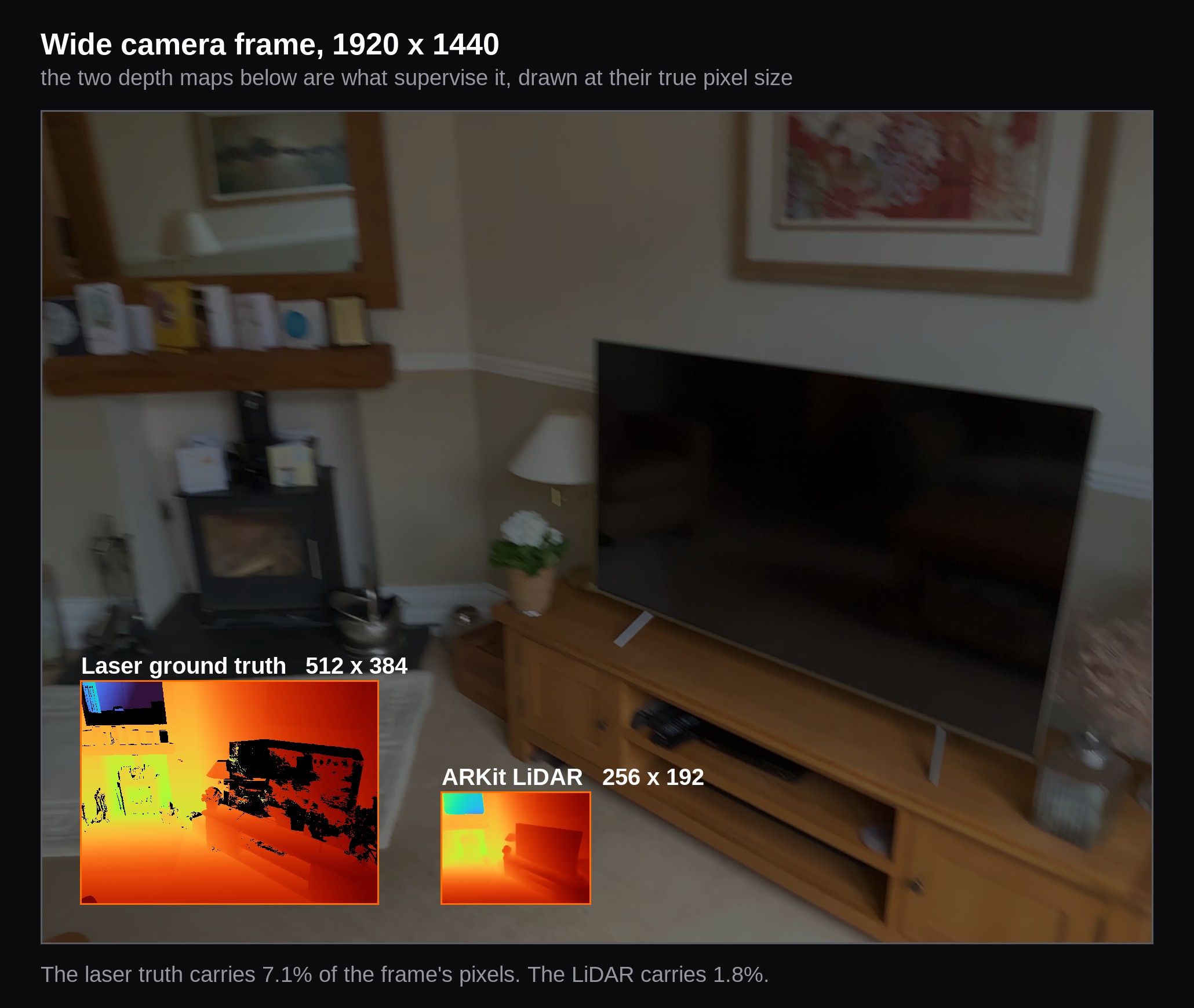
PromptDA combines the low-resolution ARKit depth with cues from high-resolution RGB, so it can predict values where the laser scanner returned nothing. In this frame, valid laser pixels give us a local check on those predictions.
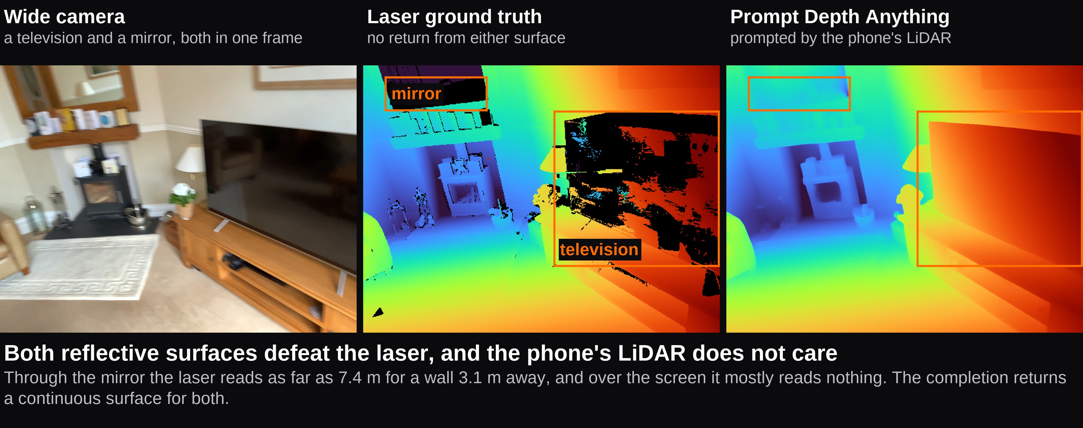
It can also repair places where the laser has no good return, such as the television above. It is not a cure for every sensor failure. Where the phone's prompt is confidently wrong, the completion inherits some of that error.
The post processing pipeline
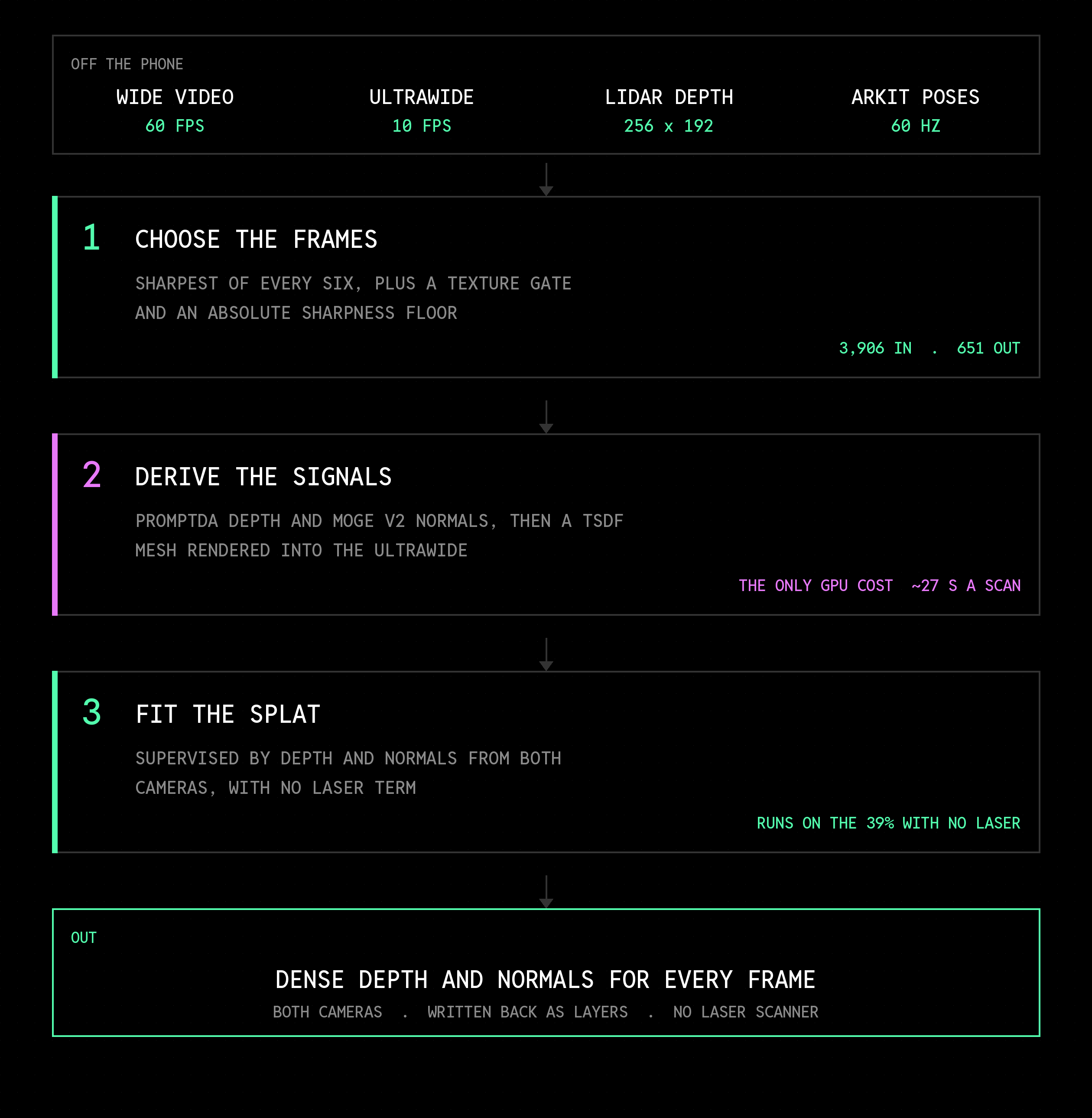
The post processing pipeline we want to build converts the original data into a candidate pseudo-label product. It runs in three stages per scan: choose the frames, derive the signals, and fit the splat. Each output stays queryable on the same timeline as the evidence that produced it, rather than becoming a folder of rendered images that must be matched back to the scan later.
Stage 1: choose the frames
Frame selection is a label-quality decision. Blurred frames poison both the splat and anything trained on its renders. We score every wide frame by the variance of its Laplacian, the same number used earlier, and keep the sharpest frame out of every six. The wide camera runs at 60 fps, so that still leaves 10 frames a second. The paper never picks two frames within six of each other either, so this is its spacing at the fastest allowed rate. It used far fewer frames because Zip-NeRF only needed a couple of hundred good views. Whether a splat benefits from more views remains an evaluation question. It might do better with fewer, sharper frames, in which case the threshold matters more than the rate.
Because the score is just a scalar on video_time, it lands in the recording beside the video it describes and the viewer plots the two together.
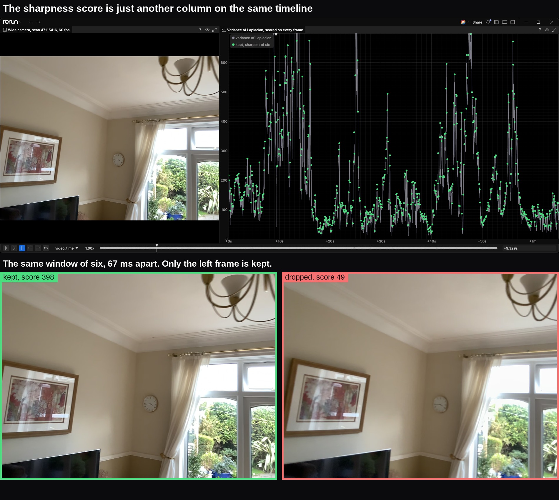
Two kinds of bad frame still get through. A blank wall is as smooth as a blurred photo, so a frame also has to have some detail in it to count. And picking the best of six says nothing about whether that best is any good, so a fixed sharpness threshold drops it if it is still blurry. Between them, a bad stretch of a scan contributes nothing rather than contributing junk.
Then require at least 200 frames to survive. At 10 per second that is 20 seconds of usable capture, which throws out the shortest 1% of scans, the ones too brief to see a room from enough angles to reconstruct it. The median scan is 65 seconds and yields around 650 frames, so the floor costs almost nothing. It only looks generous because of the rate: at the paper's 2 per second the same floor would have cut three quarters of the corpus.
The ultrawide gets its own scores, since its exposure and shake differ from the wide camera's. At 10 fps it is already at the target rate, so it skips the best-of-six step: every frame that clears the sharpness threshold is kept. Fewer frames clear it than on the wide camera.
Stage 2: derive the signals
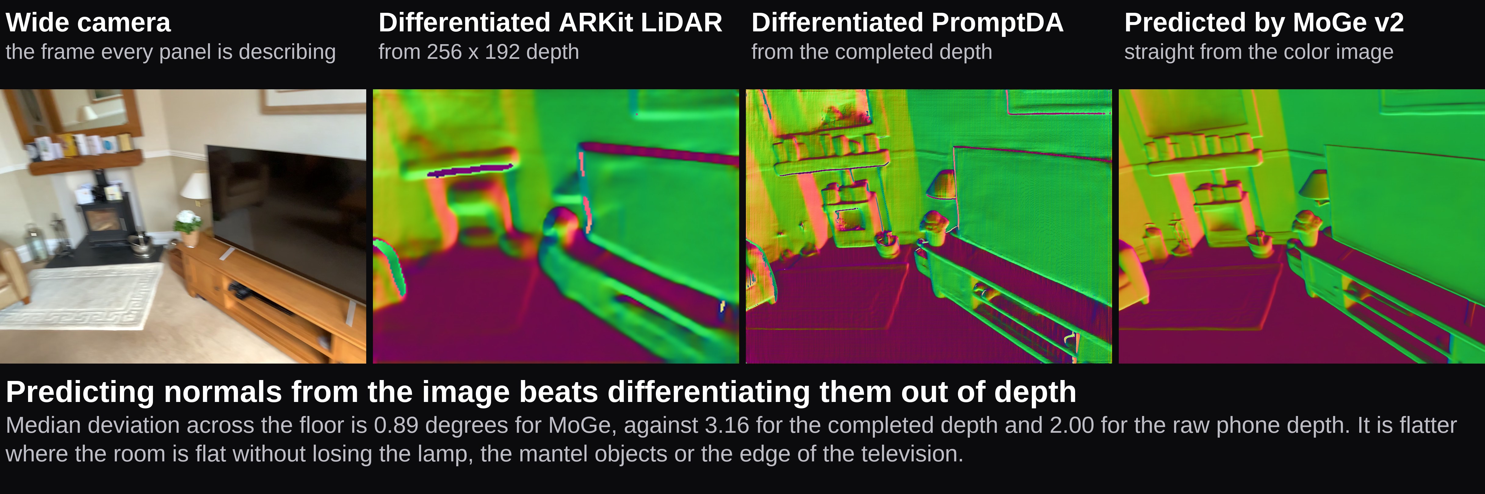
The two models contribute different evidence. PromptDA contributes dense metric depth, anchored by the phone's own LiDAR prompt. MoGe v2 contributes an independent surface normal from the color image. Keeping those signals independent matters because agreement can support a label while disagreement can become a confidence signal.
Run PromptDA on the chosen wide frames. Mask low-confidence LiDAR returns out of the prompt. The model clamps each output to the range measured by LiDAR in that frame. This per-frame clamp preserves metric scale, but it can clip the far field differently from frame to frame. Store each result at 1008×756, the network's native prediction resolution. A 1920×1440 version would only be a bilinear upsample and would use four times the storage.
MoGe v2 predicts surface normals directly from the color image. We could differentiate normals from the PromptDA depth, but that would reweight a signal the depth loss already carries. Image-derived normals provide a second opinion instead. That is why DN-Splatter and VCR-Gauss both use a separate normal network indoors.
The normals make that case better than the depth maps do.
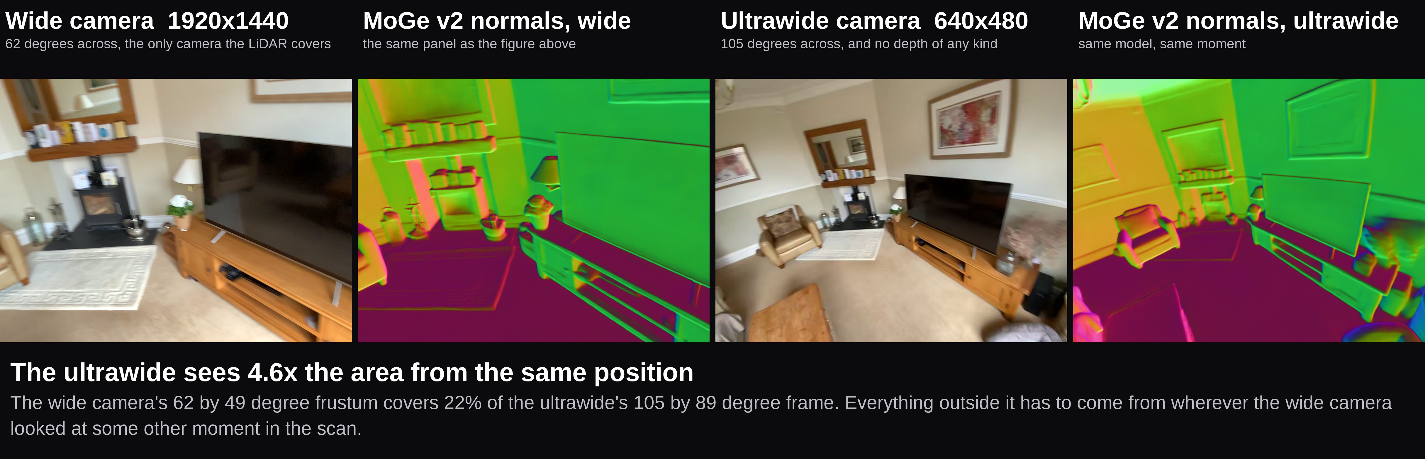
The wide depth is then TSDF-fused into a single mesh with the poses and intrinsics already in the recording. That mesh supplies initial supervision for the ultrawide by being rasterized into each ultrawide pose. Rendering the accumulated mesh is more useful than warping one frame's LiDAR prompt across. A single prompt covers only 22.5% of the ultrawide frame because the LiDAR's 62 degree cone is much narrower than the ultrawide's 105 degree field of view.
The ultrawide matters for training because it is a second lens with a much wider view and no original labels of any kind. Its labels can cover surfaces that the wide camera crops away. The TSDF render initializes those labels, but the splat fitted in Stage 3 is the part that reconciles predictions in one shared scene and makes the final outputs consistent across views. It is also what enables final candidate depth to be rendered into the ultrawide at all. Coverage then depends on where the wide camera looked during the whole trajectory, rather than where it looked in one frame.
It is worth seeing how much the wider lens provides.
Stage 3: fit the splat
Supervise one Gaussian splat with depth and normals from both cameras, using the masked normal losses from GausSurf: a term against the MoGe prior, a consistency term against the depth-derived normal, and a NeuRIS-style gate that drops the prior wherever it contradicts the rendered surface. The splat is one scene representation rather than a collection of independent frame predictions, so its renders are cross-view consistent by construction. There is no laser term in the fit, which lets this stage run on the scans that have no laser at all. Where a laser scan does exist, we hold it out for evaluation.
Put together, one scan looks like this:
def process(seg_id: str) -> None:
    seg = dataset.filter_segments(seg_id)
    wide, ultrawide, lidar, poses = read(seg)   # decode once, 7.6 s

    # Stage 1: best of every six, not every sixth
    sharp = [variance_of_laplacian(f) for f in wide]
    chosen = [sharpest(w, sharp) for w in windows(len(wide), 6)]
    chosen = [i for i in chosen
              if sharp[i] > FLOOR and has_texture(wide[i])]
    if len(chosen) < 200:
        return                        # under 20 s of usable capture

    # the ultrawide is only 10 fps, so nothing to throw away
    chosen_uw = [i for i, f in enumerate(ultrawide)
                 if variance_of_laplacian(f) > FLOOR]

    # Stage 2: the only per-frame GPU cost, ~27 s for a median scan
    depth = promptda(wide[chosen],
                     prompt=mask_by_confidence(lidar[chosen]))
    normals = moge(wide[chosen])      # an opinion, not a derivative

    mesh = tsdf_fuse(depth, poses.wide[chosen], K_wide,
                     clip=PER_FRAME_MAX)
    uw_depth = render(mesh, poses.uw[chosen_uw], undistort(K_uw))
    uw_normals = moge(ultrawide[chosen_uw])

    # Stage 3: no laser term, so this runs on laser-less scans too
    splat = train(wide[chosen], ultrawide[chosen_uw],
                  depth, normals, uw_depth, uw_normals)
Together, these stages produce a dense candidate pseudo-label layer for each chosen view. Density is immediate; accuracy still has to be measured.
At roughly 27 seconds of PromptDA plus MoGe per median scan, 100 segments is about an hour of inference, so splat training is what actually gates this rather than the networks. The plan is to walk it up: one segment, then ten, then a hundred once it trains fast enough on the one 5090.
Registering the new data as layers
A derived label should not overwrite the measurement that produced it. The raw LiDAR, laser depth, PromptDA prediction, splat render, sharpness score, and confidence masks are evidence with different failure modes. Writing them as layers lets a dataloader or viewer join them at the same timestamp. We can train on one target, compare it with another, filter bad frames, and trace a prediction back to its inputs without copying the scan into a new dataset for every experiment.
A layer is a recording with the same recording id as the segment. Layers merge on query, so a row written at time t lands beside the video sample already at t. A training query can select RGB as the input, a PromptDA or splat render as the target, sharpness and confidence as filters, and laser-valid pixels as a held-out metric, all from one segment. Changing the target or filter changes the query rather than rebuilding the dataset.
Eight named layers carry the selection, the derived signals, and the splat products:
| Layer | What it holds |
|---|---|
frame_selection | sharpness for every frame, and which ones survived |
promptda | wide depth at 1008×756, and the TSDF mesh fused from it |
moge_normals | wide normals |
ultrawide_depth | mesh depth rendered into the rectified ultrawide |
ultrawide_normals | MoGe v2 on the ultrawide frames |
splat | the trained Gaussian splat |
splat_depth | depth rendered from the splat, for both cameras |
splat_triage | per-frame error maps against the references: RGB, depth, normal angle |
Writing the layer is two columnar calls and a registration:
# plain ints are read as seconds, so cast
t = t_ns.astype("timedelta64[ns]")

with rr.RecordingStream(APP_ID, recording_id=seg_id) as rec:
    rec.save(rrd_path)

    # dense: a score for every frame, so it plots under the video
    rr.send_columns(
        f"{CAM_00}/video/sharpness",
        indexes=[rr.TimeColumn("video_time", duration=t)],
        columns=rr.Scalars.columns(scalars=sharp),
    )
    # sparse: emitting only at the chosen frames is the selection
    rr.send_columns(
        "/frame_selection/wide/chosen",
        indexes=[rr.TimeColumn("video_time", duration=t[chosen])],
        columns=rr.AnyValues.columns(
            sharpness=sharp[chosen], window=windows, rule=rules
        ),
    )

dataset.register(
    [rrd_path.as_uri()], layer_name="frame_selection"
).wait()
The Final Data after post processing
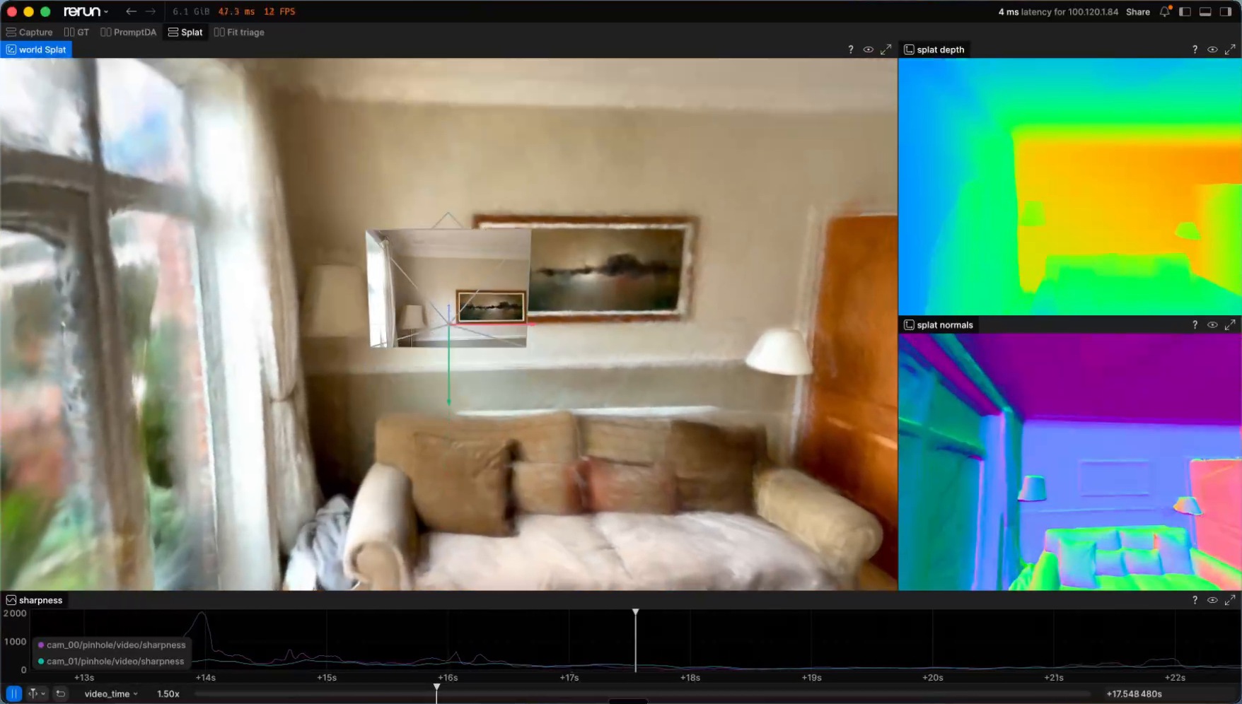
Finally after running the full pipeline, we end with a dense, metrically accurate reconstruction of the scene. We now have dense depth that avoids many of the pitfalls described in the blog above. Multiview consistent and high resolution geometry along with a gaussian splat as the final output shown in the video below for the ultrawide camera (which, in the original dataset, had no depth or surface normal ground truth).
There are still some issues, such as overly smoothed regions in some of the depth/normal maps, missing fine details in some of the geometry, and incorrect values for certain reflective regions such as the windows/mirrors. But overall, the quality of the labels dramatically improved and, critically, WITHOUT the need for FARO laser scans. This gives us a good foundation for pseudo GT for the other half of scans that did not include laser scans and, even more importantly, for in-the-wild captures for anyone with an iPhone Pro!
Conclusion: On to Network Finetuning and Training
Now that we've gone and augmented the data for higher quality labels, the next step in our journey is going to be to do some data curation and finally network training. We need to go through and query the data looking for any issues that may affect the downstream network training, such as failures in the ARKit pose estimates. Bad depth outputs from splat training, or segments with too many reflective surfaces using multiview geometry as a filter. With a filtered dataset we can finally start doing some network evaluation, finetuning and training! We'll explore this in the next blog post.
References
- apple/ARKitScenes: the dataset.
- rerun/arkitscenes-rrd: the converted corpus.
- arkitscenes-download: the conversion pipeline.
- prompt-da: the depth upsampling run.